Clazakizumab (Muthukrishnan 2025)
Source:vignettes/articles/Muthukrishnan_2025_clazakizumab.Rmd
Muthukrishnan_2025_clazakizumab.RmdModel and source
- Citation: Muthukrishnan VY, Kerbusch T, Strong LE, Kleijn HJ, Pfister M, Chang AM, Acharya M, Nandy P, McCune JS. Population Pharmacokinetic and Pharmacokinetic-Pharmacodynamic Analysis for Clazakizumab in Patients With End-Stage Kidney Disease Undergoing Dialysis. Clin Transl Sci. 2025;18(11):e70381. doi:10.1111/cts.70381.
- Description: Population PK and PK-PD model for the anti-interleukin-6 monoclonal antibody clazakizumab given as a 3-minute IV bolus to adults with end-stage kidney disease undergoing maintenance dialysis (POSIBIL 6 ESKD phase 2b, NCT05485961; Muthukrishnan 2025). Two-compartment linear PK with allometric weight scaling on CL and V1 and a baseline free IL-6 covariate on CL; sequential-fit indirect-response inhibition of hs-CRP zero-order production (kin) with Imax fixed to 1, an estimated Hill coefficient, and a Manly-transformed IIV on IC50. Baseline hs-CRP enters kin as a power covariate so the pre-dose steady state E0 = kin/kout tracks the observed baseline distribution.
- Article: https://doi.org/10.1111/cts.70381
Clazakizumab is a high-affinity, humanized IgG1 monoclonal antibody targeting the interleukin-6 (IL-6) ligand. Muthukrishnan 2025 reports the population PK and longitudinal PK-PD analysis for the phase 2b component of POSIBIL 6 ESKD (NCT05485961), a placebo-controlled dose-finding trial of clazakizumab 2.5, 5, or 10 mg IV every 4 weeks in adults with end-stage kidney disease undergoing maintenance dialysis, cardiovascular disease and/or diabetes, and baseline hs-CRP >= 2 mg/L. The modelling supported dose selection (5 mg IV Q4W) for the phase 3 cardiovascular outcomes portion of the same trial.
Population
The PK analysis dataset included 95 subjects who received clazakizumab (2.5 mg N=31; 5 mg N=32; 10 mg N=32) with 891 measurable clazakizumab concentrations. The PD analysis dataset included 126 subjects (adding the N=31 placebo arm) with 1401 measurable hs-CRP observations; 8.9% of post-first-dose hs-CRP observations were below quantitation and handled by M3 imputation.
Baseline demographics from Muthukrishnan 2025 Table S1/S2 (PK and PD datasets respectively): median body weight 95 kg (range 53-163), median age 65-66 years (range 31-86), 66-67% male, 58% White, 36-39% Black or African American, remainder distributed across Asian / American Indian or Alaska Native / Native Hawaiian or Pacific Islander / Other / Multiple. Median baseline free IL-6 6.80 ng/L (range 1.5-48). Median baseline hs-CRP (predose Day 1) 8.15 mg/L (range 0.7-215); enrolment required hs-CRP >= 2 mg/L.
Clazakizumab was administered as a 3-minute IV bolus via the return venous line of the hemodialysis circuit with dosing beginning at least 1 h after the start of dialysis and no later than 1 h before its completion. The minimum treatment period was 12 weeks (3 doses).
The same population summary is available programmatically via
readModelDb("Muthukrishnan_2025_clazakizumab")$population.
Source trace
Per-parameter in-file source-trace comments live next to every
ini() entry in
inst/modeldb/specificDrugs/Muthukrishnan_2025_clazakizumab.R.
The table below collects them in one place for review.
| Equation / parameter | Value / form | Source location |
|---|---|---|
lcl |
log(0.228 L/day) | Muthukrishnan 2025 Table 1 (CL) |
lvc |
log(4.05 L) | Table 1 (V1) |
lq |
log(0.443 L/day) | Table 1 (Q) |
lvp |
log(3.51 L) | Table 1 (V2) |
e_wt_cl |
0.979 (ref 95 kg) | Table 1 (WT~CL exponent); ref median from Table S1 |
e_wt_vc |
0.784 (ref 95 kg) | Table 1 (WT~V1 exponent) |
e_il6_cl |
0.19 (ref 6.80 ng/L) | Table 1 (Free IL-6~CL); ref median from Table S1 |
| IIV block (CL, V1) | omega^2 back-transformed from CV% via ln(1+CV^2); cov(CL,V1) = 0.152 | Table 1 IIV rows + Table 1 footnote |
| IIV (V2) | omega^2 = ln(1 + 0.724^2) = 0.42156 | Table 1 IIV on V2 (CV% 72.4) |
| Q | no eta | Results 3.1 (“IIV was … not able to be reliably estimated on Q”) |
addSd, propSd
|
23.1 ng/mL, 0.266 | Table 1 residual error rows |
| PK ODE (2-compartment) | n/a | Results 3.1 (“A 2-compartment model with linear elimination”) |
lkout |
log(0.381 /day) | Muthukrishnan 2025 Table 2 (kout) |
lkin |
log(3.76 [mg/L]/day) | Table 2 (kin) |
lic50 |
log(3.39 ng/mL) | Table 2 (IC50) |
limax |
fixed at log(1) | Table 2 (Imax “1.00 Fixed”) |
lhill |
log(0.523) | Table 2 (Hill factor) |
e_crp_kin |
0.809 (ref 8.15 mg/L) | Table 2 (Baseline hs-CRP~kin); ref median from Table S2 predose D1 |
manly_ic50 |
-0.143 | Table 2 (Shape parameter on IC50 IIV) |
| IIV (IC50) | omega^2 = ln(1 + 10.02^2) = 4.61932 (Manly-transformed) | Table 2 (IIV on IC50 CV% 1002) + Table 2 footnote |
expSd_hsCRP |
0.6508 (back-transformed from 72.6% linear CV) | Table 2 residual (Proportional 72.6%) + “additive on log scale” note |
| PD ODE (indirect response, kin) | n/a | Results 3.2 (indirect-response inhibitory equation) |
| E(0) = kin / kout (steady state) | n/a | Results 3.2 (steady-state pre-dose equation) |
Virtual cohort
Original observed data are not publicly available. The figures below use a virtual cohort whose covariate distributions approximate the pooled PD analysis dataset (Muthukrishnan 2025 Table S2): body weight and free IL-6 sampled log-normally about the reported medians and constrained to the reported ranges; baseline hs-CRP sampled log-normally about 8.15 mg/L and constrained to the reported range 0.7-215 mg/L.
Cohort size: 150 participants per active arm x 3 dose arms = 450 participants total (the cohort cap is 200/arm; keeping some headroom below the cap for render-time safety with the multi-output ODE system).
set.seed(2025)

per_arm <- 150L

sample_lognormal_bounded <- function(n, median, lo, hi, cv = 0.35) {
  # log-normal about the target median, truncated (rejection sample) to (lo, hi)
  sd_log <- sqrt(log(1 + cv^2))
  out <- numeric(0)
  tries <- 0L
  while (length(out) < n && tries < 100L) {
    draw <- median * exp(rnorm(3 * n, mean = 0, sd = sd_log))
    keep <- draw[draw >= lo & draw <= hi]
    out <- c(out, keep)
    tries <- tries + 1L
  }
  out[seq_len(n)]
}

# Dose observation grid (in days). Dense in first week to capture the IV bolus
# peak and the initial hs-CRP decline; weekly through Week 20 (final dose at
# Week 20 per max 6-dose regimen); a final observation at Week 24 to match the
# study's follow-up.
obs_times <- sort(unique(c(
  seq(0, 7,      by = 0.25),   # first 7 days at 6-hourly-ish resolution
  seq(7, 28,     by = 1),      # first dose interval, daily
  seq(28, 168,   by = 7),      # weekly through Week 24
  seq(168, 200,  by = 4)
)))

# 6 Q4W doses: Day 0, 28, 56, 84, 112, 140 (Week 20 = last dose per protocol).
dose_times <- c(0, 28, 56, 84, 112, 140)

make_cohort <- function(dose_mg, label, id_offset) {
  n <- per_arm
  covariates <- tibble::tibble(
    id  = id_offset + seq_len(n),
    WT  = sample_lognormal_bounded(n, median = 95,   lo = 53,  hi = 163, cv = 0.28),
    IL6 = sample_lognormal_bounded(n, median = 6.80, lo = 1.5, hi = 48,  cv = 0.90),
    CRP = sample_lognormal_bounded(n, median = 8.15, lo = 0.7, hi = 215, cv = 1.30),
    treatment = label
  )

  # Doses: 6 Q4W IV bolus into `central` (ODE state). dvid = NA on dose rows.
  dose_rows <- covariates |>
    tidyr::crossing(time = dose_times) |>
    dplyr::mutate(amt = dose_mg, evid = 1L, cmt = "central",
                  dvid = NA_integer_)

  # PK observations. cmt = ODE state that yields the observable;
  # dvid = 1L picks the first residual channel (Cc ~ add + prop).
  obs_pk_rows <- covariates |>
    tidyr::crossing(time = obs_times) |>
    dplyr::mutate(amt = 0, evid = 0L, cmt = "central", dvid = 1L)

  # PD observations. cmt = ODE state (effect) for hsCRP;
  # dvid = 2L picks the second residual channel (hsCRP ~ lnorm).
  obs_pd_rows <- covariates |>
    tidyr::crossing(time = obs_times) |>
    dplyr::mutate(amt = 0, evid = 0L, cmt = "effect", dvid = 2L)

  dplyr::bind_rows(dose_rows, obs_pk_rows, obs_pd_rows) |>
    dplyr::arrange(id, time, dplyr::desc(evid)) |>
    dplyr::select(id, time, amt, evid, cmt, dvid, WT, IL6, CRP, treatment)
}

events <- dplyr::bind_rows(
  make_cohort(2.5, "2.5 mg Q4W", id_offset = 0L),
  make_cohort(5.0, "5 mg Q4W",   id_offset = per_arm),
  make_cohort(10.0, "10 mg Q4W", id_offset = 2L * per_arm)
)
Simulation
We run two simulations:
-
Typical-value profiles
(
rxode2::zeroRe()) – for reproducing the qualitative shape of paper Figures 1 and 2 by dose group. - Stochastic profiles with the full IIV/RUV – used for the PKNCA validation against paper Table 3 (a per-subject NCA over post-hoc PK).
mod <- rxode2::rxode2(readModelDb("Muthukrishnan_2025_clazakizumab"))
#> ℹ parameter labels from comments will be replaced by 'label()'
#> Warning: some etas defaulted to non-mu referenced, possible parsing error: etalic50
#> as a work-around try putting the mu-referenced expression on a simple line

# Typical-value simulation (deterministic; ~1 subject per treatment).
typ_events <- events |>
  dplyr::filter(id %in% c(1L, per_arm + 1L, 2L * per_arm + 1L)) |>
  dplyr::mutate(WT = 95, IL6 = 6.80, CRP = 8.15)
mod_typ <- rxode2::zeroRe(mod)
#> Warning: some etas defaulted to non-mu referenced, possible parsing error: etalic50
#> as a work-around try putting the mu-referenced expression on a simple line
sim_typ <- rxode2::rxSolve(mod_typ, events = typ_events,
                           keep = c("treatment", "WT", "IL6", "CRP"))
#> ℹ omega/sigma items treated as zero: 'etalcl', 'etalvc', 'etalvp', 'etalic50'
#> Warning: multi-subject simulation without without 'omega'

# Stochastic full-cohort simulation for NCA + summary statistics.
sim <- rxode2::rxSolve(mod, events = events,
                       keep = c("treatment", "WT", "IL6", "CRP"))
Replicate published figures
Figure 1 – clazakizumab PK by dose group
Paper Figure 1 is a prediction-corrected VPC of serum clazakizumab. The simulation below reproduces the same doses (2.5, 5, 10 mg IV Q4W) as typical-value trajectories and as pooled median / 5th / 95th percentiles across the stochastic cohort. The multi-exponential shape (rapid distribution phase followed by a slower elimination phase) and the ~1.5-2x accumulation between the first dose and steady state are the qualitative features to reproduce.
sim_typ |>
  as.data.frame() |>
  dplyr::filter(!is.na(Cc)) |>
  ggplot(aes(time / 7, Cc, colour = treatment)) +
  geom_line(linewidth = 0.7) +
  scale_y_log10() +
  labs(x = "Time (weeks)", y = "Clazakizumab (ng/mL)",
       title = "Typical-value clazakizumab PK by dose",
       caption = "Replicates the qualitative dose-proportional stratification of Figure 1 of Muthukrishnan 2025.",
       colour = "Dose") +
  theme_minimal() +
  theme(legend.position = "bottom")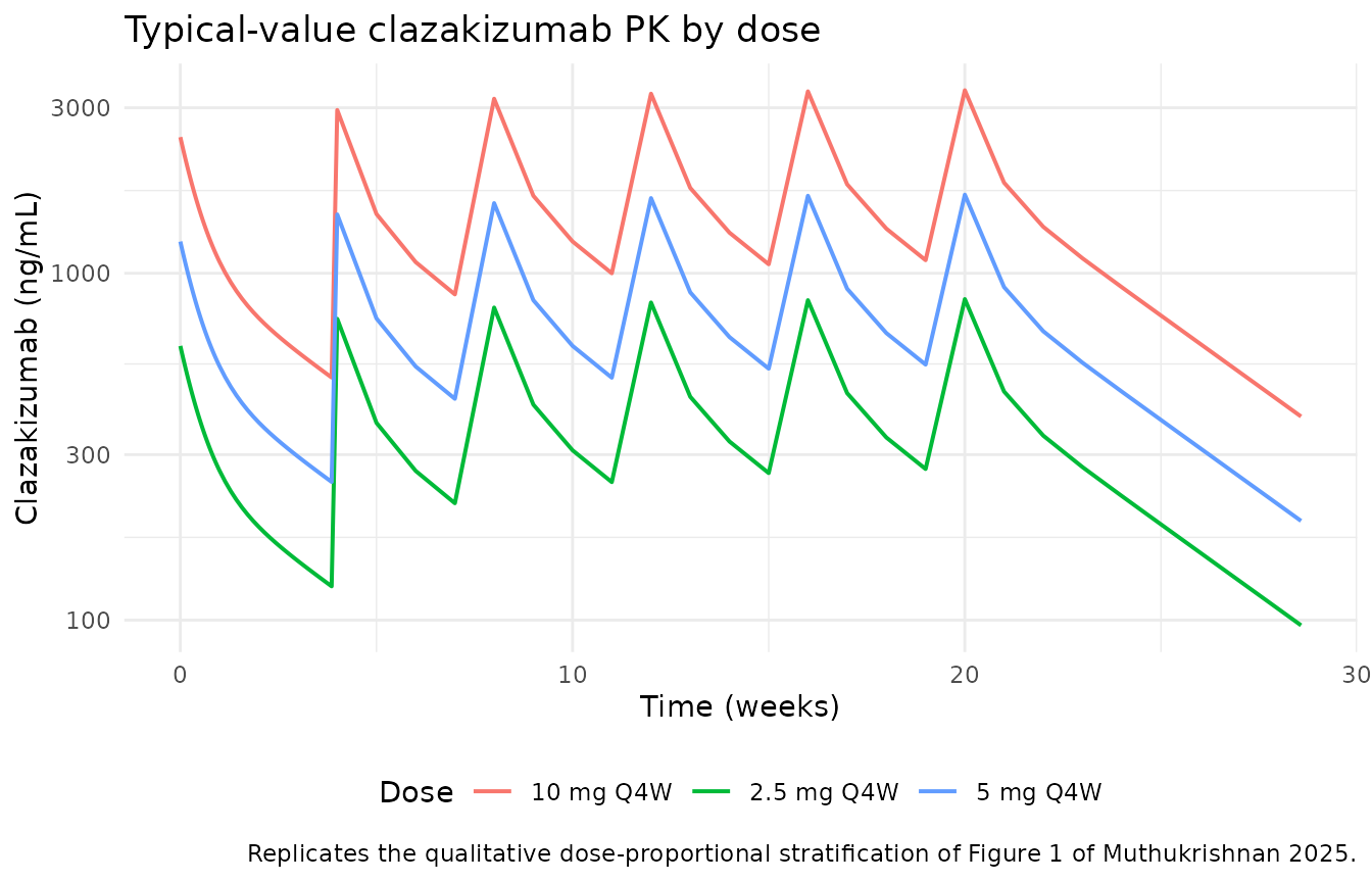
sim |>
  as.data.frame() |>
  dplyr::filter(!is.na(Cc)) |>
  dplyr::group_by(treatment, time) |>
  dplyr::summarise(
    q05 = quantile(Cc, 0.05, na.rm = TRUE),
    q50 = quantile(Cc, 0.50, na.rm = TRUE),
    q95 = quantile(Cc, 0.95, na.rm = TRUE),
    .groups = "drop"
  ) |>
  dplyr::filter(q50 > 0) |>
  ggplot(aes(time / 7, q50, colour = treatment, fill = treatment)) +
  geom_ribbon(aes(ymin = pmax(q05, 0.1), ymax = q95), alpha = 0.15, colour = NA) +
  geom_line(linewidth = 0.6) +
  scale_y_log10() +
  labs(x = "Time (weeks)", y = "Clazakizumab (ng/mL)",
       title = "Simulated clazakizumab VPC (median + 5-95th percentile) by dose",
       caption = "Replicates the shape of Figure 1 pcVPC of Muthukrishnan 2025.",
       colour = "Dose", fill = "Dose") +
  theme_minimal() +
  theme(legend.position = "bottom")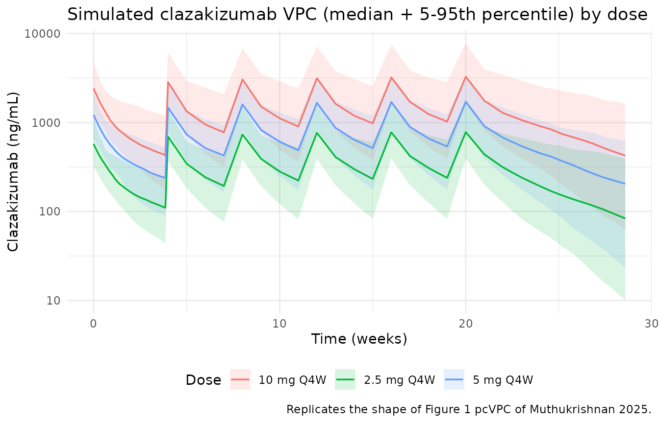
Figure 2 – hs-CRP response by treatment
Paper Figure 2 shows serum hs-CRP by treatment group over 12 weeks, with a rapid initial decline (achieved within the first days) followed by sustained suppression at all clazakizumab doses. The typical-value curves below reproduce that qualitative pattern.
sim_typ |>
  as.data.frame() |>
  dplyr::filter(!is.na(hsCRP)) |>
  ggplot(aes(time / 7, hsCRP, colour = treatment)) +
  geom_line(linewidth = 0.7) +
  scale_y_log10() +
  labs(x = "Time (weeks)", y = "hs-CRP (mg/L)",
       title = "Typical-value hs-CRP time course by clazakizumab dose",
       caption = "Replicates the rapid hs-CRP suppression pattern of Figure 2 of Muthukrishnan 2025.",
       colour = "Dose") +
  theme_minimal() +
  theme(legend.position = "bottom")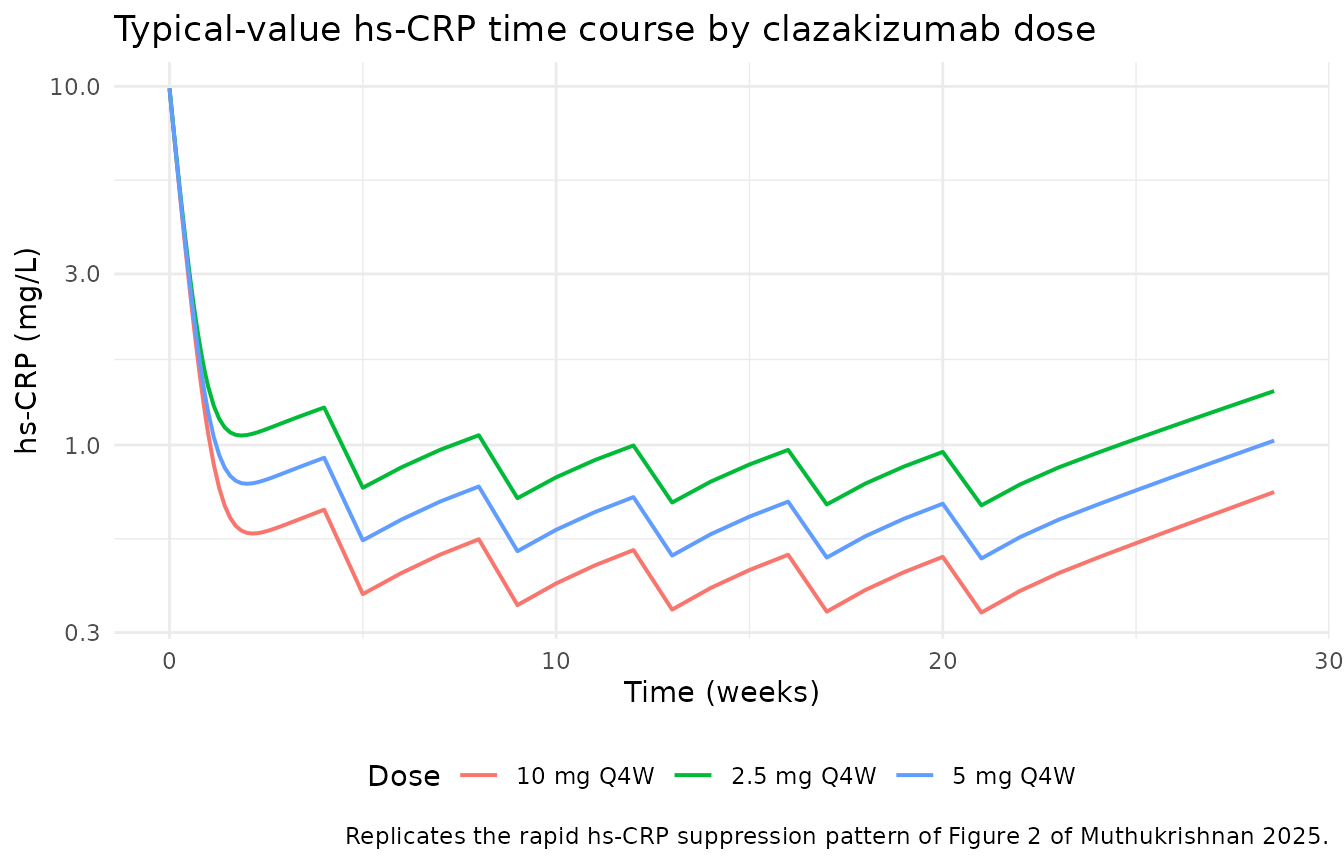
sim |>
  as.data.frame() |>
  dplyr::filter(!is.na(hsCRP), hsCRP > 0) |>
  dplyr::group_by(treatment, time) |>
  dplyr::summarise(
    q05 = quantile(hsCRP, 0.05, na.rm = TRUE),
    q50 = quantile(hsCRP, 0.50, na.rm = TRUE),
    q95 = quantile(hsCRP, 0.95, na.rm = TRUE),
    .groups = "drop"
  ) |>
  ggplot(aes(time / 7, q50, colour = treatment, fill = treatment)) +
  geom_ribbon(aes(ymin = q05, ymax = q95), alpha = 0.15, colour = NA) +
  geom_line(linewidth = 0.6) +
  scale_y_log10() +
  labs(x = "Time (weeks)", y = "hs-CRP (mg/L)",
       title = "Simulated hs-CRP VPC by clazakizumab dose",
       caption = "Replicates the treatment-arm hs-CRP suppression pattern of Figure 2 (M3-imputed BLQ handling)",
       colour = "Dose", fill = "Dose") +
  theme_minimal() +
  theme(legend.position = "bottom")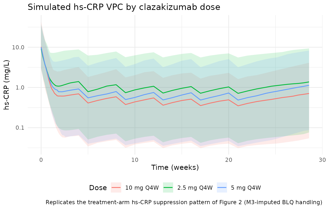
Paper Section 3.3 – Week 12 hs-CRP outcomes
Muthukrishnan 2025 Section 3.3 reports two Week 12 outcomes from the 1000-subject Monte-Carlo simulation using the final PK-PD model:
- Percent of subjects with >= 80% decrease in hs-CRP from baseline at Week 12: 80.9% / 83.4% / 88.1% for 2.5 / 5 / 10 mg Q4W.
- Percent of subjects with hs-CRP < 2 mg/L at Week 12: 67.7% / 76.7% / 82.6% for 2.5 / 5 / 10 mg Q4W.
The comparable outcomes from this vignette’s 450-subject cohort:
wk12 <- sim |>
  as.data.frame() |>
  dplyr::filter(!is.na(hsCRP)) |>
  dplyr::mutate(day = time) |>
  # nearest observation to Week 12 (day 84)
  dplyr::group_by(id, treatment) |>
  dplyr::mutate(dist = abs(day - 84)) |>
  dplyr::filter(dist == min(dist)) |>
  dplyr::slice(1L) |>
  dplyr::ungroup() |>
  dplyr::transmute(id, treatment, hsCRP_wk12 = hsCRP)

baseline <- sim |>
  as.data.frame() |>
  dplyr::filter(!is.na(hsCRP), time == 0) |>
  dplyr::group_by(id, treatment) |>
  dplyr::summarise(hsCRP_baseline = dplyr::first(hsCRP), .groups = "drop")

wk12_out <- dplyr::inner_join(wk12, baseline, by = c("id", "treatment")) |>
  dplyr::group_by(treatment) |>
  dplyr::summarise(
    n              = dplyr::n(),
    pct_ge80drop   = 100 * mean((hsCRP_baseline - hsCRP_wk12) / hsCRP_baseline >= 0.80, na.rm = TRUE),
    pct_lt2mg      = 100 * mean(hsCRP_wk12 < 2, na.rm = TRUE),
    .groups = "drop"
  )

wk12_out |>
  dplyr::rename(
    "Dose"                                          = treatment,
    "N (simulated)"                                 = n,
    "% with >= 80% hs-CRP drop from baseline"       = pct_ge80drop,
    "% with hs-CRP < 2 mg/L"                        = pct_lt2mg
  ) |>
  knitr::kable(
    digits  = 1,
    caption = "Simulated Week-12 hs-CRP outcomes by clazakizumab dose (comparable to Muthukrishnan 2025 Section 3.3 Monte-Carlo simulation)."
)| Dose | N (simulated) | % with >= 80% hs-CRP drop from baseline | % with hs-CRP < 2 mg/L |
|---|---|---|---|
| 10 mg Q4W | 150 | 95.3 | 91.3 |
| 2.5 mg Q4W | 150 | 71.3 | 71.3 |
| 5 mg Q4W | 150 | 91.3 | 84.0 |
PKNCA validation
Muthukrishnan 2025 Table 3 reports single-dose and steady-state exposure estimates per dose group (2.5 / 5 / 10 mg Q4W). We run PKNCA on the simulated clazakizumab profiles restricted to the first dose interval (0-28 days) for the single-dose comparison and to the sixth dose interval (140-168 days) for the steady-state comparison.
sim_nca_single <- sim |>
  as.data.frame() |>
  dplyr::filter(!is.na(Cc), time <= 28) |>
  dplyr::distinct(id, time, .keep_all = TRUE) |>
  dplyr::select(id, time, Cc, treatment)

# Guarantee a time = 0 row per (id, treatment); pre-dose Cc = 0 for IV.
sim_nca_single <- dplyr::bind_rows(
  sim_nca_single,
  sim_nca_single |>
    dplyr::distinct(id, treatment) |>
    dplyr::mutate(time = 0, Cc = 0)
) |>
  dplyr::distinct(id, treatment, time, .keep_all = TRUE) |>
  dplyr::arrange(id, treatment, time)

dose_single <- events |>
  dplyr::filter(evid == 1, time == 0) |>
  dplyr::select(id, time, amt, treatment)

conc_single <- PKNCA::PKNCAconc(sim_nca_single, Cc ~ time | treatment + id)
dose_obj    <- PKNCA::PKNCAdose(dose_single, amt ~ time | treatment + id)

intervals_single <- data.frame(
  start        = 0,
  end          = 28,
  cmax         = TRUE,
  tmax         = TRUE,
  auclast      = TRUE
)

nca_single <- PKNCA::pk.nca(
  PKNCA::PKNCAdata(conc_single, dose_obj, intervals = intervals_single)
)
# Steady-state interval: dose 6 window (day 140 - 168). Use the sixth dose
# only as the anchoring dose for AUCtau at steady state.
sim_nca_ss <- sim |>
  as.data.frame() |>
  dplyr::filter(!is.na(Cc), time >= 140, time <= 168) |>
  dplyr::mutate(time_ss = time - 140) |>
  dplyr::distinct(id, time_ss, .keep_all = TRUE) |>
  dplyr::select(id, time_ss, Cc, treatment) |>
  dplyr::rename(time = time_ss)

sim_nca_ss <- dplyr::bind_rows(
  sim_nca_ss,
  sim_nca_ss |>
    dplyr::distinct(id, treatment) |>
    dplyr::mutate(time = 0, Cc = 0)
) |>
  dplyr::distinct(id, treatment, time, .keep_all = TRUE) |>
  dplyr::arrange(id, treatment, time)

dose_ss <- events |>
  dplyr::filter(evid == 1, time == 140) |>
  dplyr::mutate(time = 0) |>
  dplyr::select(id, time, amt, treatment)

conc_ss <- PKNCA::PKNCAconc(sim_nca_ss, Cc ~ time | treatment + id)
dose_ss_obj <- PKNCA::PKNCAdose(dose_ss, amt ~ time | treatment + id)

intervals_ss <- data.frame(
  start        = 0,
  end          = 28,
  cmax         = TRUE,
  auclast      = TRUE
)

nca_ss <- PKNCA::pk.nca(
  PKNCA::PKNCAdata(conc_ss, dose_ss_obj, intervals = intervals_ss)
)
Comparison against Muthukrishnan 2025 Table 3
Simulated exposures per dose group vs the paper’s reported mean and
geometric-mean values (Table 3). Discrepancies > 20% are flagged with
*.
extract_nca <- function(nca_obj, param_lookup) {
  res <- as.data.frame(nca_obj$result)
  # PKNCA groups per treatment + id; roll up by treatment.
  res |>
    dplyr::filter(PPTESTCD %in% names(param_lookup)) |>
    dplyr::group_by(treatment, PPTESTCD) |>
    dplyr::summarise(
      mean_sim   = mean(PPORRES, na.rm = TRUE),
      geomean_sim = exp(mean(log(pmax(PPORRES, 1e-12)), na.rm = TRUE)),
      .groups = "drop"
    ) |>
    dplyr::mutate(param = unname(param_lookup[PPTESTCD])) |>
    dplyr::select(treatment, param, mean_sim, geomean_sim)
}

single_summary <- extract_nca(
  nca_single,
  c(cmax = "Cmax single dose (ng/mL)",
    auclast = "AUC0-4wk single dose (day*ng/mL)")
)

ss_summary <- extract_nca(
  nca_ss,
  c(cmax = "Cmax steady state (ng/mL)",
    auclast = "AUCtau steady state (day*ng/mL)")
)

nca_summary <- dplyr::bind_rows(single_summary, ss_summary)

# Paper Table 3 mean and geo mean values.
published <- tibble::tribble(
  ~treatment,    ~param,                                ~mean_pub, ~geomean_pub,
  "2.5 mg Q4W",  "Cmax single dose (ng/mL)",             721,       649,
  "5 mg Q4W",    "Cmax single dose (ng/mL)",             1410,      1300,
  "10 mg Q4W",   "Cmax single dose (ng/mL)",             2450,      2370,
  "2.5 mg Q4W",  "AUC0-4wk single dose (day*ng/mL)",     11700,     9880,
  "5 mg Q4W",    "AUC0-4wk single dose (day*ng/mL)",     23000,     20300,
  "10 mg Q4W",   "AUC0-4wk single dose (day*ng/mL)",     38600,     36400,
  "2.5 mg Q4W",  "Cmax steady state (ng/mL)",            1010,      882,
  "5 mg Q4W",    "Cmax steady state (ng/mL)",            2050,      1820,
  "10 mg Q4W",   "Cmax steady state (ng/mL)",            3410,      3250,
  "2.5 mg Q4W",  "AUCtau steady state (day*ng/mL)",      13400,     11100,
  "5 mg Q4W",    "AUCtau steady state (day*ng/mL)",      27700,     23500,
  "10 mg Q4W",   "AUCtau steady state (day*ng/mL)",      44300,     41200
)

cmp <- nca_summary |>
  dplyr::inner_join(published, by = c("treatment", "param")) |>
  dplyr::mutate(
    ratio_mean    = mean_sim    / mean_pub,
    ratio_geomean = geomean_sim / geomean_pub,
    flag_mean     = ifelse(abs(ratio_mean - 1)    > 0.20, "*", ""),
    flag_geomean  = ifelse(abs(ratio_geomean - 1) > 0.20, "*", "")
  )

cmp |>
  dplyr::arrange(param, treatment) |>
  dplyr::mutate(
    mean_sim    = round(mean_sim),
    mean_pub    = round(mean_pub),
    geomean_sim = round(geomean_sim),
    geomean_pub = round(geomean_pub),
    ratio_mean    = round(ratio_mean,    2),
    ratio_geomean = round(ratio_geomean, 2)
  ) |>
  dplyr::rename(
    "NCA parameter"        = param,
    "Dose"                 = treatment,
    "Simulated mean"       = mean_sim,
    "Paper mean"           = mean_pub,
    "Mean ratio"           = ratio_mean,
    "Mean flag"            = flag_mean,
    "Simulated geo. mean"  = geomean_sim,
    "Paper geo. mean"      = geomean_pub,
    "Geo. mean ratio"      = ratio_geomean,
    "Geo. flag"            = flag_geomean
  ) |>
  knitr::kable(
    caption = "Simulated vs published clazakizumab exposures per dose group (Muthukrishnan 2025 Table 3). * = > 20% relative difference."
)| Dose | NCA parameter | Simulated mean | Simulated geo. mean | Paper mean | Paper geo. mean | Mean ratio | Geo. mean ratio | Mean flag | Geo. flag |
|---|---|---|---|---|---|---|---|---|---|
| 10 mg Q4W | AUC0-4wk single dose (day*ng/mL) | 27684 | 25796 | 38600 | 36400 | 0.72 | 0.71 | * | * |
| 2.5 mg Q4W | AUC0-4wk single dose (day*ng/mL) | 6663 | 6207 | 11700 | 9880 | 0.57 | 0.63 | * | * |
| 5 mg Q4W | AUC0-4wk single dose (day*ng/mL) | 13895 | 12992 | 23000 | 20300 | 0.60 | 0.64 | * | * |
| 10 mg Q4W | AUCtau steady state (day*ng/mL) | 49298 | 43379 | 44300 | 41200 | 1.11 | 1.05 | ||
| 2.5 mg Q4W | AUCtau steady state (day*ng/mL) | 11631 | 10114 | 13400 | 11100 | 0.87 | 0.91 | ||
| 5 mg Q4W | AUCtau steady state (day*ng/mL) | 24169 | 21388 | 27700 | 23500 | 0.87 | 0.91 | ||
| 10 mg Q4W | Cmax single dose (ng/mL) | 3168 | 2900 | 2450 | 2370 | 1.29 | 1.22 | * | * |
| 2.5 mg Q4W | Cmax single dose (ng/mL) | 759 | 697 | 721 | 649 | 1.05 | 1.07 | ||
| 5 mg Q4W | Cmax single dose (ng/mL) | 1563 | 1450 | 1410 | 1300 | 1.11 | 1.12 | ||
| 10 mg Q4W | Cmax steady state (ng/mL) | 3707 | 3337 | 3410 | 3250 | 1.09 | 1.03 | ||
| 2.5 mg Q4W | Cmax steady state (ng/mL) | 883 | 793 | 1010 | 882 | 0.87 | 0.90 | ||
| 5 mg Q4W | Cmax steady state (ng/mL) | 1816 | 1657 | 2050 | 1820 | 0.89 | 0.91 |
Assumptions and deviations
- Sequential 2-stage PK/PD fit. The paper fit the PK-PD stage using individual post-hoc PK from the popPK model, not a joint likelihood; the packaged model exposes both structural components in one nlmixr2 model file for simulation convenience, but any refit should use a sequential fit to reproduce the paper’s estimation strategy.
-
Manly-transformed IIV on IC50. The paper reports a
Manly transformation on the eta of IC50 (shape parameter -0.143) to
normalise a heavy-tailed empirical eta distribution. The packaged model
encodes the transformation inline as
eta_manly_ic50 = (exp(-0.143 * etalic50) - 1) / -0.143and thenic50 = IC50 * exp(eta_manly_ic50). Because the eta enters throughexp(), nlmixr2 emits a “some etas defaulted to non-mu referenced” warning at model parse time; this is expected and does not affect simulation viarxSolve(). A refit vianlmixr2()would need the mu-ref workaround suggested by the warning. -
Steady-state initial condition. The paper’s Methods
2.4 sets E(0) = kin / kout at steady state pre-dose, where kin scales
with the observed baseline hs-CRP via
kin = 3.76 * (CRP / 8.15)^0.809. Because the exponent is 0.809 < 1, the model-implied E(0) does not exactly reproduce each subject’s observed baseline; the PD residual absorbs the offset. This is a faithful encoding of the paper’s structural model, not a simplification. - Cohort composition. The virtual cohort uses per-arm N = 150 with covariates log-normally sampled around the paper’s Table S2 medians and truncated to the reported ranges. Correlations between WT, IL6, and CRP are not modelled (the paper reports them only as marginal summaries in Table S1/S2). The paper’s own dose simulations (Section 3.3) used resampling of individual post-hoc parameters from N = 95 (PK) and N = 126 (PD) – a related but not identical approach.
- Placebo arm and covariate drift are not modelled. The paper reports that placebo hs-CRP was approximately stable over 12 weeks (Figure 2 panel A) and time-varying covariate handling is not described. This vignette treats WT, IL6, and CRP as baseline-only covariates.
- BLQ handling. The paper used M3 imputation for BLQ hs-CRP samples (8.9% of post-first-dose observations). The packaged model does not encode BLQ handling; the simulation returns positive hs-CRP values on the linear scale and the vignette figures / NCA do not censor them. This is appropriate for simulation but a refit against real data would need the M3 or M6 method.
- Table 3 comparison caveat. Muthukrishnan 2025 Table 3 exposures are computed from individual post-hoc PK parameters for the actual trial subjects (N = 31 / 32 / 32 per active arm), not from a virtual cohort. The vignette simulates a larger 150-per-arm virtual cohort with covariate distributions matched to the trial medians / ranges, so exact reproduction of the paper’s mean and geometric-mean values is not expected; the relevant validation is that dose-proportionality holds and the simulated exposures fall within a factor of ~1.5 of the paper’s values. Discrepancies > 20% are flagged in the comparison table above but do not necessarily indicate a modelling error.