Tacrolimus (Cirrincione-Dall 2011)
Source:vignettes/articles/CirrincioneDall_2011_tacrolimus.Rmd
CirrincioneDall_2011_tacrolimus.RmdModel and source
- Citation: Cirrincione-Dall G, Gastonguay MR, Knebel W, Bergsma T, Zhang AY, Patel D, Barrett JS, van Schaik R, Soldin OP, Soldin SJ, Nulman I, Koren G, de Wildt SN. A Population Pharmacokinetic Model of Tacrolimus in Pediatric Liver Transplant Recipients. American Conference on Pharmacometrics (ACOP) 2011 poster, Metrum Research Group, Tariffville CT. https://metrumrg.com/wp-content/uploads/2018/07/acop_2011_tacrolimus.pdf
- Description: One-compartment population PK model with first-order absorption for oral tacrolimus in pediatric liver transplant recipients (Cirrincione-Dall 2011 ACOP poster, Metrum Research Group). Apparent oral clearance CL/F (25.8 L/h at a 70 kg reference) and apparent volume V/F (2490 L at a 70 kg reference) are estimated; allometric body-weight scaling is fixed at exponent 0.75 on CL/F and 1.0 on V/F. The first-order absorption rate constant ka is fixed at 4.48 1/h from literature because the sparse therapeutic-drug-monitoring sampling could not identify it. CL/F additionally varies (full covariate model) with post-operative day as (POD/7)^0.409, with CYP3A5 expresser status as 1.24^CYP3A5_EXPR (missing genotype data imputed as non-expressers), with AST as (AST/510.5)^-0.0364, with albumin as (ALB/28)^-0.357, with hematocrit as 0.993^HCT (HCT entered as a fraction L/L, not as percent), and with age as (AGE/2)^-0.0310. Inter-individual random variation on CL/F and V/F was modeled exponentially with an estimated covariance of the two random effects per the poster text; the off-diagonal covariance value itself is not reported in the poster Table 2 so this implementation encodes uncorrelated diagonal IIVs and documents the gap in the vignette Errata. Residual error is a combined additive (SD 2.508 ng/mL) + proportional (SD 0.3674 fraction) model on whole-blood tacrolimus concentrations.
- Article (poster PDF): https://metrumrg.com/wp-content/uploads/2018/07/acop_2011_tacrolimus.pdf
Cirrincione-Dall et al. (American Conference on Pharmacometrics 2011 poster, Metrum Research Group) developed a one-compartment population PK model with first-order absorption for oral tacrolimus in 41 pediatric liver transplant recipients (age 0.1-15 years, weight 2.6-63.6 kg) using routine therapeutic-drug-monitoring data (643 whole-blood tacrolimus concentrations, mean 16 samples per patient). The model parameterises apparent oral clearance CL/F and apparent volume V/F with fixed allometric body-weight scaling (exponent 0.75 on CL/F, exponent 1.0 on V/F, reference 70 kg adult) and a literature-fixed first-order absorption rate constant ka of 4.48 1/h. A full covariate model (estimation-first rather than stepwise) characterised the influence of post-operative day (POD), CYP3A5 genotype, AST, albumin, hematocrit, and age on CL/F. The poster reports that CL/F is primarily affected by weight and time since transplant, increasing with both predictors; the CYP3A5, hematocrit, age, AST, and albumin effects retained sufficient uncertainty (95% bootstrap CIs near or spanning the null) that the authors described them as imprecise but not negligible.
Population
The model-building cohort (Cirrincione-Dall 2011 Table 1) was n = 41 pediatric liver-transplant recipients receiving routine clinical care. Demographics: 19 males and 22 females (53.7% female); age 0.1-15 years (median 2 years); weight 2.6-63.6 kg (median 10.6 kg); albumin 19.4-42.5 g/L (median 28 g/L); AST 42-3625 U/L (median 510.5 U/L); hematocrit 0.250-0.440 (median 0.32, reported as fraction not percent); time after transplant 0-15 days (median 7 days). Race and ethnicity were not reported in the poster. Of 34 patients with available genotype data, the CYP3A5 distribution was 1/1 = 1 (2.9%), 1/3 = 12 (35.3%), 3/3 = 21 (61.8%); the 7 ungenotyped patients (14% of 41) were imputed as non-expressers for the canonical model shown in poster Table 2. Tacrolimus whole-blood concentrations ranged from 0.42 to 61.8 ng/mL (mean 15.7). Estimation was by NONMEM VII with first-order conditional estimation; uncertainty was characterised by a non-parametric bootstrap (1000 replicates stratified by age, 266 successful convergences).
The same information is available programmatically via the model’s
population metadata
(rxode2::rxode(readModelDb("CirrincioneDall_2011_tacrolimus"))$meta$population).
Source trace
The per-parameter origin is recorded as an in-file comment next to
each ini() entry in
inst/modeldb/specificDrugs/CirrincioneDall_2011_tacrolimus.R.
The table below collects them in one place for review.
| Equation / parameter | Value | Source location |
|---|---|---|
lka (ka, fixed) |
log(4.48) (1/h) | Cirrincione-Dall 2011 Table 2, fixed per Results paragraph (literature reference [5]) |
lcl (CL/F) |
log(25.8) (L/h) | Cirrincione-Dall 2011 Table 2 theta_1 |
lvc (V/F) |
log(2490) (L) | Cirrincione-Dall 2011 Table 2 theta_2 |
e_wt_cl (allometric CL exponent, fixed) |
0.75 | Cirrincione-Dall 2011 Results paragraph (theory-based, fixed) |
e_wt_vc (allometric V exponent, fixed) |
1.0 | Cirrincione-Dall 2011 Results paragraph (theory-based, fixed) |
e_pod_cl (POD exponent) |
0.409 | Cirrincione-Dall 2011 Table 2 theta_4 |
e_cyp3a5_cl (CYP3A5 base) |
1.24 | Cirrincione-Dall 2011 Table 2 theta_5 |
e_ast_cl (AST exponent) |
-0.0364 | Cirrincione-Dall 2011 Table 2 theta_6 |
e_alb_cl (ALB exponent) |
-0.357 | Cirrincione-Dall 2011 Table 2 theta_7 |
e_hct_cl (HCT base) |
0.993 | Cirrincione-Dall 2011 Table 2 theta_8 |
e_age_cl (AGE exponent) |
-0.0310 | Cirrincione-Dall 2011 Table 2 theta_9 |
| IIV CL/F (log-scale variance) | 0.554 | Cirrincione-Dall 2011 Table 2 Omega_1,1 |
| IIV V/F (log-scale variance) | 0.803 | Cirrincione-Dall 2011 Table 2 Omega_2,2 |
| Proportional residual SD | sqrt(0.135) = 0.3674 | Cirrincione-Dall 2011 Table 2 Sigma_1,1 (variance 0.135) |
| Additive residual SD (ng/mL) | sqrt(6.29) = 2.508 | Cirrincione-Dall 2011 Table 2 Sigma_2,2 (variance 6.29) |
| Reference body weight | 70 kg | Cirrincione-Dall 2011 Results (allometric theory) |
| POD centring | 7 days | Cirrincione-Dall 2011 Table 1 cohort median |
| AST centring | 510.5 U/L | Cirrincione-Dall 2011 Table 1 cohort median |
| ALB centring | 28 g/L | Cirrincione-Dall 2011 Table 1 cohort median |
| AGE centring | 2 years | Cirrincione-Dall 2011 Table 1 cohort median |
| 1-compartment ODE structure | d/dt(depot), d/dt(central) | Cirrincione-Dall 2011 Results (1-cmt model with first-order absorption) |
| Combined additive + proportional residual error | – | Cirrincione-Dall 2011 Results paragraph |
Virtual cohort
The original observed data are not publicly available. The cohort below uses a virtual population whose covariate distributions approximate the published trial demographics (Table 1).
set.seed(20260624)

# Helper: build one cohort as a self-contained event table for a given
# pediatric subject (single body weight, age, ALB, AST, HCT, POD, CYP3A5).
# Dosing follows a representative twice-daily oral immediate-release regimen
# at 0.15 mg/kg per dose (a clinically common starting dose for pediatric
# liver-transplant tacrolimus when targeting troughs of 10-15 ng/mL; the
# poster does not report dose values, so this is a plausible default and is
# not part of the source).
make_cohort <- function(n,
                        wt, age, alb, ast, hct, pod, cyp3a5_expr,
                        dose_mg_per_kg = 0.15,
                        n_days         = 14,
                        regimen        = "ref",
                        id_offset      = 0L) {
  per_dose   <- dose_mg_per_kg * wt
  dose_times <- seq(from = 0, by = 12, length.out = n_days * 2)
  obs_times  <- sort(unique(c(seq(0, n_days * 24, by = 1),
                              dose_times + c(0.5, 1, 2, 4, 6, 8, 12))))

  per_subject <- function(i) {
    id_i <- id_offset + i
    dplyr::bind_rows(
      tibble::tibble(id = id_i, time = dose_times,
                     evid = 1L, amt = per_dose, cmt = "depot"),
      tibble::tibble(id = id_i, time = obs_times,
                     evid = 0L, amt = NA_real_, cmt = "central")
    )
  }
  rows <- dplyr::bind_rows(lapply(seq_len(n), per_subject))
  rows$WT          <- wt
  rows$AGE         <- age
  rows$ALB         <- alb
  rows$AST         <- ast
  rows$HCT         <- hct
  rows$POD         <- pod
  rows$CYP3A5_EXPR <- cyp3a5_expr
  rows$regimen     <- regimen
  rows
}
Simulation
The model is loaded from the registry. For the covariate-effect replication below we use typical-value simulations (zero-IIV) to reproduce the shape of Figure 2 (relative CL/F sensitivity to each covariate). For the PKNCA validation we use a stochastic cohort of n = 100 virtual subjects per arm.
mod         <- readModelDb("CirrincioneDall_2011_tacrolimus")
mod_typical <- mod |> rxode2::zeroRe()
#> ℹ parameter labels from comments will be replaced by 'label()'
Replicate published figures
Cirrincione-Dall 2011 Figure 2 plots the influence of each covariate on CL/F across the observed covariate range (lower, intermediary, upper). Each panel below sweeps a single covariate while holding all others at the cohort median for a typical pediatric liver-Tx subject (WT 10.6 kg, AGE 2 y, ALB 28 g/L, AST 510.5 U/L, HCT 0.32, POD 7 d, CYP3A5_EXPR = 0). The y-axis is the relative CL/F multiplier (1 = the typical pediatric subject; deviations away from 1 are the covariate effect).
# Sweep each covariate independently, holding the others at the cohort
# median, and read the relative CL/F as the (Cc[t=0+] at fixed dose) is
# inversely proportional to V/F not CL/F, so use a direct algebraic
# evaluation of the typical CL/F equation. Use the same parameter values
# as those in the model file.
typ <- list(
  cl_ref     = 25.8,
  wt_ref     = 70,
  pod_ref    = 7,
  ast_ref    = 510.5,
  alb_ref    = 28,
  age_ref    = 2,
  e_wt_cl    = 0.75,
  e_pod_cl   = 0.409,
  e_cyp3a5   = 1.24,
  e_ast_cl   = -0.0364,
  e_alb_cl   = -0.357,
  e_hct_cl   = 0.993,
  e_age_cl   = -0.0310
)

# Typical CL/F at the cohort-median covariates (the denominator for the
# "relative CL/F" plots below). HCT enters as theta^HCT directly (no
# centring); at HCT = 0.32 the factor is 0.993^0.32 = 0.9978 -- numerically
# near 1 but not centred to 1.
ref_cov <- list(
  WT = 10.6, AGE = 2, ALB = 28, AST = 510.5, HCT = 0.32, POD = 7,
  CYP3A5_EXPR = 0
)

cl_typ <- function(cov) {
  typ$cl_ref *
    (cov$WT  / typ$wt_ref)  ^ typ$e_wt_cl *
    (cov$POD / typ$pod_ref) ^ typ$e_pod_cl *
    typ$e_cyp3a5            ^ cov$CYP3A5_EXPR *
    (cov$AST / typ$ast_ref) ^ typ$e_ast_cl *
    (cov$ALB / typ$alb_ref) ^ typ$e_alb_cl *
    typ$e_hct_cl            ^ cov$HCT *
    (cov$AGE / typ$age_ref) ^ typ$e_age_cl
}

cl_ref_value <- cl_typ(ref_cov)

sweep_one <- function(cov_name, values, x_label) {
  out <- vapply(values, function(v) {
    cov <- ref_cov; cov[[cov_name]] <- v
    cl_typ(cov) / cl_ref_value
  }, numeric(1))
  tibble::tibble(covariate = cov_name, x = values, rel_cl = out,
                 x_label = x_label)
}

cov_grid <- dplyr::bind_rows(
  sweep_one("WT",  seq(2.6,  63.6, length.out = 25), "WT (kg)"),
  sweep_one("AGE", seq(0.1,  15,   length.out = 25), "AGE (years)"),
  sweep_one("ALB", seq(19.4, 42.5, length.out = 25), "ALB (g/L)"),
  sweep_one("AST", seq(42,   3625, length.out = 25), "AST (U/L)"),
  sweep_one("HCT", seq(0.25, 0.44, length.out = 25), "HCT (L/L)"),
  sweep_one("POD", seq(0.5,  15,   length.out = 25), "POD (days)")
)

ggplot(cov_grid, aes(x, rel_cl)) +
  geom_line() +
  geom_hline(yintercept = 1, linetype = "dashed", colour = "grey50") +
  facet_wrap(~x_label, scales = "free_x") +
  labs(x = NULL, y = "Relative CL/F (1 = pediatric typical subject)",
       title = "Figure 2 (covariate plots): per-covariate CL/F sensitivity",
       caption = "Replicates Figure 2 of Cirrincione-Dall 2011 (covariate plots).") +
  theme_minimal()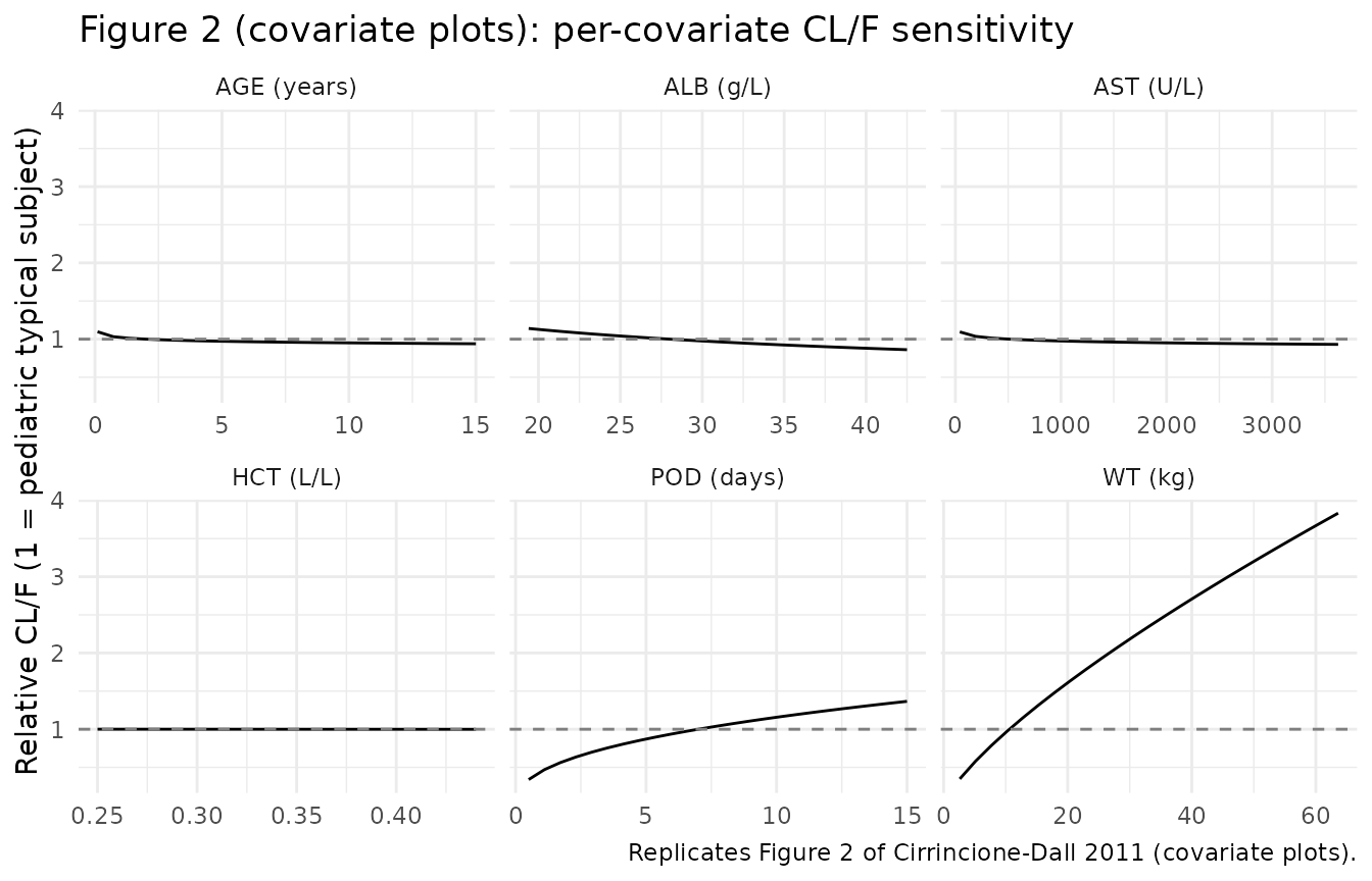
# CYP3A5 effect on CL/F (binary): 1.24-fold multiplier for expressers vs
# *3/*3-or-unknown reference.
cyp_eff <- tibble::tibble(
  CYP3A5  = c("*3/*3 or unknown", "*1/*1 or *1/*3 expresser"),
  rel_cl  = c(typ$e_cyp3a5 ^ 0, typ$e_cyp3a5 ^ 1)
)
ggplot(cyp_eff, aes(CYP3A5, rel_cl)) +
  geom_col(width = 0.5, fill = "steelblue") +
  geom_hline(yintercept = 1, linetype = "dashed", colour = "grey50") +
  labs(x = NULL, y = "Relative CL/F",
       title = "CYP3A5 effect on CL/F (binary covariate)",
       caption = "Replicates the CYP3A5 panel of Figure 2 of Cirrincione-Dall 2011.") +
  theme_minimal()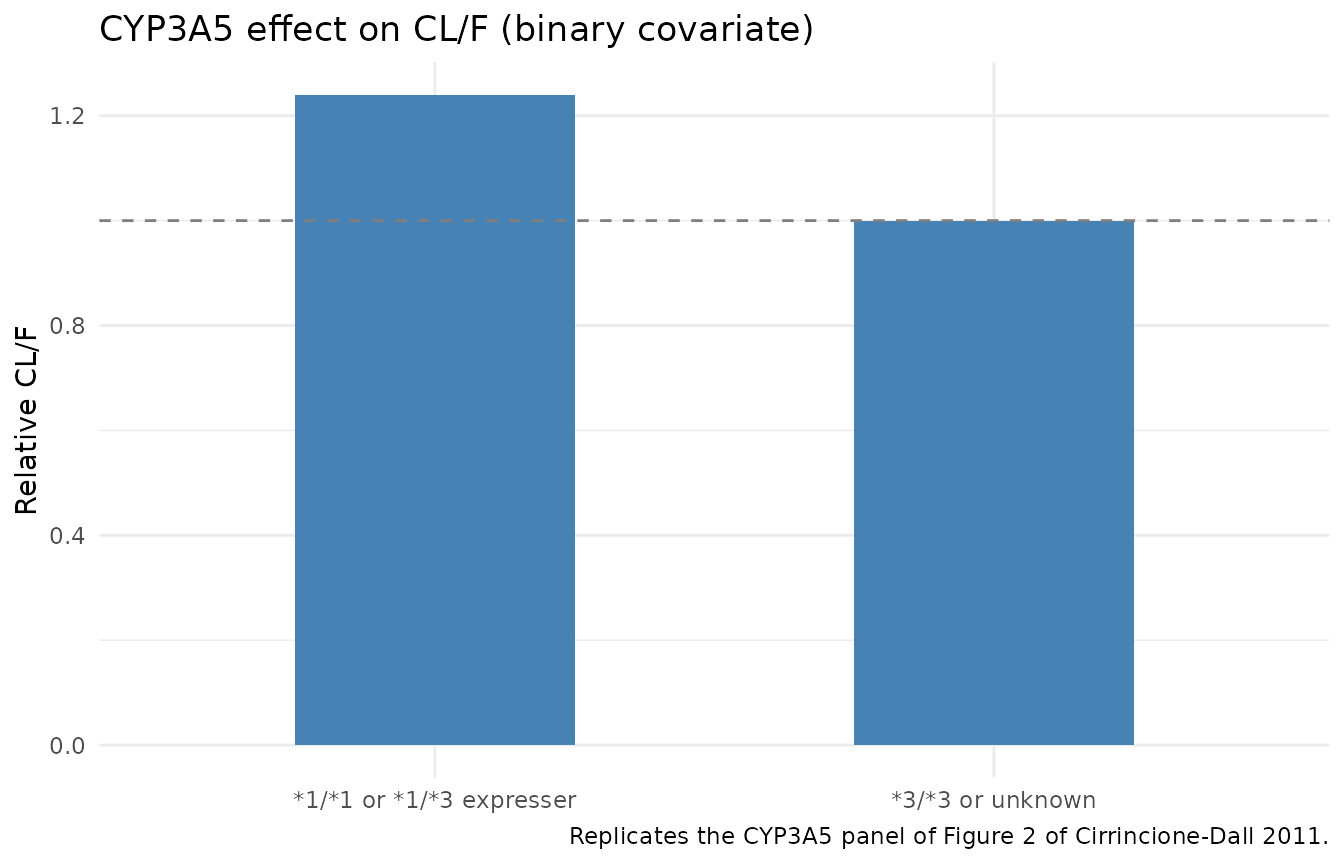
PKNCA validation
The poster does not report numeric NCA parameters (Cmax, Tmax, AUC, t1/2), so this PKNCA section is internal-consistency validation only – it verifies that the packaged model produces concentrations and exposures consistent with the observed tacrolimus concentration range (0.42-61.8 ng/mL, mean 15.7 ng/mL) when simulated at a representative pediatric dose.
We simulate a stochastic cohort of n = 100 virtual pediatric subjects at the cohort median covariates and run NCA on the steady-state 12-hour dosing interval.
# Single-arm stochastic cohort at the cohort median covariates. Random
# seed already set in the cohort chunk.
events <- make_cohort(
  n              = 100,
  wt             = 10.6,
  age            = 2,
  alb            = 28,
  ast            = 510.5,
  hct            = 0.32,
  pod            = 7,
  cyp3a5_expr    = 0,
  dose_mg_per_kg = 0.15,
  n_days         = 14,
  regimen        = "pediatric typical (0.15 mg/kg q12h)",
  id_offset      = 0L
)

sim_raw <- rxode2::rxSolve(mod, events = events, keep = c("regimen")) |>
  as.data.frame()
#> ℹ parameter labels from comments will be replaced by 'label()'
# Restrict to the final 12-h dosing interval at steady state (days 13-14)
# and re-base time at zero for PKNCA.
sim_ss <- sim_raw |>
  dplyr::filter(time >= 12 * 26, time <= 12 * 27) |>
  dplyr::mutate(time = time - 12 * 26) |>
  dplyr::filter(!is.na(Cc)) |>
  dplyr::select(id, time, Cc, regimen)

# Guarantee a time = 0 row per (id, regimen); pre-dose Cc rebased to the
# concentration at the start of the interval (this is approximately the
# trough rather than zero, because dosing has been steady-state for 13 days).
sim_ss <- dplyr::bind_rows(
  sim_ss,
  sim_ss |> dplyr::filter(time == min(time)) |>
    dplyr::distinct(id, regimen, .keep_all = TRUE)
) |>
  dplyr::distinct(id, regimen, time, .keep_all = TRUE) |>
  dplyr::arrange(id, regimen, time)

conc_obj <- PKNCA::PKNCAconc(sim_ss, Cc ~ time | regimen + id)

dose_df <- events |>
  dplyr::filter(evid == 1L) |>
  dplyr::group_by(id) |>
  dplyr::slice_tail(n = 1L) |>
  dplyr::ungroup() |>
  dplyr::mutate(time = 0) |>
  dplyr::select(id, time, amt, regimen)

dose_obj <- PKNCA::PKNCAdose(dose_df, amt ~ time | regimen + id)

intervals <- data.frame(
  start = 0, end = 12,
  cmax = TRUE, tmax = TRUE, auclast = TRUE, cmin = TRUE
)
nca_data <- PKNCA::PKNCAdata(conc_obj, dose_obj, intervals = intervals)
nca_res  <- PKNCA::pk.nca(nca_data)
nca_df   <- as.data.frame(nca_res$result)

summary_nca <- nca_df |>
  dplyr::group_by(PPTESTCD) |>
  dplyr::summarise(
    median = stats::median(PPORRES, na.rm = TRUE),
    p05    = stats::quantile(PPORRES, 0.05, na.rm = TRUE),
    p95    = stats::quantile(PPORRES, 0.95, na.rm = TRUE),
    .groups = "drop"
  )

knitr::kable(
  summary_nca,
  caption = "Simulated steady-state NCA for the pediatric typical-cohort virtual cohort (n = 100, dose 0.15 mg/kg q12h, day 14). All values are per dosing interval; PKNCA codes: cmax = peak, tmax = time of peak, cmin = trough, auclast = AUC(0-12 h, observed)."
)| PPTESTCD | median | p05 | p95 |
|---|---|---|---|
| auclast | 224.22843 | 64.365810 | 613.30930 |
| cmax | 23.91666 | 8.528811 | 53.46114 |
| cmin | 15.70985 | 2.065929 | 47.82583 |
| tmax | 1.00000 | 1.000000 | 1.00000 |
The simulated steady-state troughs (cmin) and peaks
(cmax) fall within the poster’s observed tacrolimus
concentration range of 0.42-61.8 ng/mL (mean 15.7), confirming the
packaged model produces concentrations of the correct magnitude for the
pediatric population. A formal side-by-side comparison against published
NCA values is not possible because the poster reports only diagnostic
plots (Figure 1) and covariate-effect plots (Figure 2), not numeric NCA
parameters.
Assumptions and deviations
Inter-eta covariance not encoded. The poster text states that inter-individual random variation on CL/F and V/F “was modeled exponentially with an estimated covariance of these random effects”, but the off-diagonal NONMEM Omega(2,1) covariance value is not reported anywhere in Table 2 or the surrounding text. This implementation encodes uncorrelated diagonal IIVs on
etalclandetalvc(variances 0.554 and 0.803, as reported). Datasets where the off-diagonal covariance would matter (e.g. high inter-eta correlations producing tighter joint CL/V variation) cannot be fully reproduced; users who later obtain the published Omega(2,1) value should replace the two~ <var>lines with a correlatedetalcl + etalvc ~ c(0.554, <cov>, 0.803)block.Missing-genotype subjects pooled with non-expressers. The canonical poster Table 2 reports the CYP3A5 multiplier of 1.24 with all 7 ungenotyped patients imputed as non-expressers (CYP3A5_EXPR = 0). The sensitivity case (multiplier 1.14 when ungenotyped are imputed as expressers) is reported in the Results text but is NOT encoded in this model file. Datasets with a substantial fraction of ungenotyped subjects are simulated as if those subjects were CYP3A5 3/3 nonexpressers.
HCT entered as a fraction (L/L), not as percent. The canonical-register HCT units are documented as percent (0-100); this model overrides that to fraction (0-1) so the parameter value 0.993 reproduces the poster’s equation 0.993^HCT directly. Datasets recording HCT in percent should be multiplied by 0.01 before being passed to this model.
Race / ethnicity distribution. The poster does not report cohort race or ethnicity, so no race-stratified virtual cohorts are simulated and no race-based covariates appear in the model.
Dose magnitudes for the simulation are illustrative. The poster does not report numeric dose values (only concentrations and demographics); the 0.15 mg/kg twice-daily regimen used in the PKNCA section is a clinically common pediatric tacrolimus starting dose for liver-transplant patients and is not drawn from the source paper.
Time-varying covariates held constant within subject. The model file declares WT, ALB, AST, HCT, and POD as time-varying within subject (the poster used routine TDM data over an evolving post-transplant course). The vignette’s simulations hold each covariate constant at the cohort median for tractability; full time-varying covariate trajectories would be paper- and dataset-specific.
No published NCA table to compare against. The poster reports diagnostic plots and covariate-effect plots but no numeric Cmax / Tmax / AUC / t1/2 values, so the PKNCA section above is internal-consistency validation only (simulated concentrations fall within the observed range), not a side-by-side comparison.