Dabigatran aPTT and ECT in orthopaedic surgery (Liesenfeld 2006)
Source:vignettes/articles/Liesenfeld_2006_dabigatran.Rmd
Liesenfeld_2006_dabigatran.RmdModel and source
- Citation: Liesenfeld K-H, Schaefer HG, Troconiz IF, Tillmann C, Eriksson BI, Stangier J. Effects of the direct thrombin inhibitor dabigatran on ex vivo coagulation time in orthopaedic surgery patients: a population model analysis. Br J Clin Pharmacol. 2006 Nov;62(5):527-537. doi:10.1111/j.1365-2125.2006.02667.x. PK structure embedded for simulation convenience from Liesenfeld 2013; see modellib(‘Liesenfeld_2013_dabigatran’).
- Article: https://doi.org/10.1111/j.1365-2125.2006.02667.x
The paper develops two pharmacodynamic (PD) models for the prolongation of two coagulation tests by dabigatran in orthopaedic-surgery patients receiving oral dabigatran etexilate after total hip replacement:
-
modellib("Liesenfeld_2006_dabigatran_aPTT")– activated partial thromboplastin time (aPTT), a combined linear + Emax relationship with time-since-surgery decay on baseline and Emax. -
modellib("Liesenfeld_2006_dabigatran_ECT")– ecarin clotting time (ECT), a linear relationship whose slope decays exponentially with time-since-surgery and whose baseline also declines.
Both models share the BISTRO I population, the same observed- concentration PK driver, and the same time-since-surgery convention; the authors fitted them in separate NONMEM V runs because the optimal PD structures differ.
Population
The PD analysis used data from the BISTRO I Phase IIa multicentre, open-label, dose-escalating study (Eriksson et al., reference [8] of the source paper). Of 289 patients enrolled, 287 contributed to both analyses; the aPTT model used 4854 paired PK-PD observations and the ECT model used 5060. Patients were 35-88 years old (mean 67), weighed 49-130 kg (mean 78), and 52.6% were female (Liesenfeld 2006 Table 1). All received oral dabigatran etexilate 4-8 h after total hip replacement surgery and continued for 6-10 days at one of nine dose levels: 12.5, 25, 50, 100, 150, 200, or 300 mg twice daily, or 150 or 300 mg once daily, with 20-46 patients per dose subgroup.
The same information is available programmatically via
readModelDb("Liesenfeld_2006_dabigatran_aPTT")$population
(and the matching ECT model).
Covariate analysis screened patient demographics (gender, age, height, body mass index), serum creatinine clearance, standard clinical laboratory parameters, and comedications (diuretics, opioids, NSAIDs, GI-transit accelerators, acetaminophen, CYP3A4 inhibitors) for effects on every PD parameter via GAM preselection followed by NONMEM forward inclusion (P = 0.05) and backward elimination (P = 0.001). None were retained in the final model (Liesenfeld 2006 Results, APTT model; Results, ECT model).
Source trace
Per-parameter origin is recorded as an in-file comment next to each
ini() entry in the model files; the tables below collect
them in one place for review.
aPTT model (Liesenfeld 2006 Table 2; Equations 1, 3, 4)
| Equation / parameter | Source value | nlmixr2lib ini()
|
Source location |
|---|---|---|---|
lrbase (BAS0, s) |
33.4 | log(33.4) |
Table 2 (RSE 0.63%) |
lemax (EMA0, s) |
26.9 | log(26.9) |
Table 2 (RSE 12.45%) |
lec50 (EC50, ng/mL) |
94.7 | log(94.7) |
Table 2 (RSE 17.11%) |
lslope (SLOP, s per ng/mL) |
0.0509 | log(0.0509) |
Table 2 (RSE 6.68%) |
let50 (ET50, h) |
1.62 days | log(1.62 * 24) |
Table 2 (RSE 15.99%) |
emba (EM_BA) |
0.102 | 0.102 |
Table 2 (RSE 14.41%) |
emmx (EM_MX) |
0.463 | 0.463 |
Table 2 (RSE 12.68%) |
| IIV E0 (CV 8.7%) | omega^2 = log(1 + 0.087^2) = 0.007541 | etalrbase ~ 0.007541 |
Table 2 |
| IIV Emax (CV 19.9%) | omega^2 = log(1 + 0.199^2) = 0.03884 | etalemax ~ 0.03884 |
Table 2 |
| IIV EC50 (CV 38.5%) | omega^2 = log(1 + 0.385^2) = 0.13821 | etalec50 ~ 0.13821 |
Table 2 |
| IIV SLOP (CV 15.2%) | omega^2 = log(1 + 0.152^2) = 0.02284 | etalslope ~ 0.02284 |
Table 2 |
| Residual error (proportional CV 7.55%) | 0.0755 | propSd <- 0.0755 |
Table 2 (RSE 3.53%) |
| Combined linear + Emax model | – | aPTT <- rbase_t + emax_t * Cc / (ec50 + Cc) + slope * Cc |
Equation 1 |
| Proportional inhibitory decay of baseline | – | rbase_t <- rbase * (1 - emba * t / (et50 + t)) |
Equation 3 |
| Proportional inhibitory decay of Emax | – | emax_t <- emax_0 * (1 - emmx * t / (et50 + t)) |
Equation 4 |
ECT model (Liesenfeld 2006 Table 3; Equations 2, 3, 5)
| Equation / parameter | Source value | nlmixr2lib ini()
|
Source location |
|---|---|---|---|
lrbase (BAS0, s) |
28.0 | log(28.0) |
Table 3 (RSE 0.49%) |
lslope0 (SLO0, s per ng/mL) |
0.377 | log(0.377) |
Table 3 (RSE 2.18%) |
lslope_inf (SLO_F, s per ng/mL) |
0.268 | log(0.268) |
Table 3 (RSE 1.49%) |
lkm (KM, 1/h) |
0.617 / 24 | log(0.617 / 24) |
Table 3 (KM = 0.617 day-1; table unit “h-1” is a transcription error – see Assumptions and deviations; RSE 13.55%) |
let50 (ET50, h) |
2.86 days | log(2.86 * 24) |
Table 3 (RSE 13.50%) |
emba (EM_BA) |
0.175 | 0.175 |
Table 3 (RSE 6.46%) |
| IIV E0 (CV 8.2%) | omega^2 = log(1 + 0.082^2) = 0.006700 | etalrbase ~ 0.006700 |
Table 3 |
| IIV SLOP (CV 13.7%) | omega^2 = log(1 + 0.137^2) = 0.01859 | etalslope0 ~ 0.01859 |
Table 3 |
| Residual error (proportional CV 6.63%) | 0.0663 | propSd <- 0.0663 |
Table 3 (RSE 6.83%) |
| Linear model with time-varying slope | – | ECT <- rbase_t + slope_t * Cc |
Equation 2 |
| Proportional inhibitory decay of baseline | – | rbase_t <- rbase * (1 - emba * t / (et50 + t)) |
Equation 3 |
| Bi-exponential slope decay | – | slope_t <- slope_inf + (slope0 - slope_inf) * exp(-km * t) |
Equation 5 |
Embedded PK structure
The 2006 paper does not develop a PK model – the PD layer was fitted
against observed dabigatran plasma concentrations. To make the model
self-contained for downstream simulation, both .R files
embed the two-compartment dabigatran disposition from Liesenfeld 2013
Table 2 with all PK thetas fixed:
ini() |
Liesenfeld 2013 value | Population |
|---|---|---|
lcl |
log(12.4) | CL/F, L/h |
lvc |
log(531) | V2/F, L |
lq |
log(152) | Q/F, L/h |
lvp |
log(499) | V3/F, L |
lka |
log(0.821) | ka, 1/h |
ltlag |
log(1.67) | ALAG, h (fed) |
lfdepot |
log(1.00) | F (anchor) |
See modellib("Liesenfeld_2013_dabigatran") for the
standalone PK model.
Load both models
mod_aPTT <- readModelDb("Liesenfeld_2006_dabigatran_aPTT")
mod_ECT  <- readModelDb("Liesenfeld_2006_dabigatran_ECT")
Replicate Figure 6 – ECT slope decay over time
Liesenfeld 2006 Figure 6 plots SLOP(T), the slope of the linear ECT-
concentration relationship, against time since first dose. The slope
declines mono-exponentially from SLO0 = 0.377 to
SLO_F = 0.268 s per ng/mL with rate constant
KM = 0.617 day^-1 (half-life 27 h = 1.1 day). The chunk
below evaluates Equation 5 directly so the curve can be compared against
the published Figure 6.
# Replicates Figure 6 of Liesenfeld 2006: SLOP vs time.
slope_0   <- 0.377     # SLO0  (s per ng/mL)
slope_inf <- 0.268     # SLO_F (s per ng/mL)
km_h      <- 0.617 / 24  # 1/h
times_h <- seq(0, 360, length.out = 200)
slope_curve <- tibble::tibble(
  time_h    = times_h,
  time_days = times_h / 24,
  slope     = slope_inf + (slope_0 - slope_inf) * exp(-km_h * time_h)
)
ggplot(slope_curve, aes(time_days, slope)) +
  geom_line() +
  geom_hline(yintercept = slope_inf, linetype = "dashed") +
  annotate("text", x = 14, y = slope_inf + 0.005,
           label = "SLO_F = 0.268", hjust = 1, size = 3) +
  geom_hline(yintercept = slope_0, linetype = "dotted") +
  annotate("text", x = 14, y = slope_0 - 0.005,
           label = "SLO0 = 0.377", hjust = 1, size = 3) +
  labs(x = "Time after first dose (days)",
       y = "SLOP (s per ng/mL)",
       title = "ECT slope vs time -- replicates Liesenfeld 2006 Figure 6",
       caption = "SLOP(T) = SLO_F + (SLO0 - SLO_F) * exp(-KM * T); half-life 27 h.")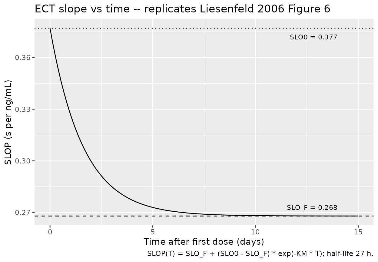
Replicate Figure 3 – aPTT Emax decay over time
Liesenfeld 2006 Figure 3 plots the time-varying Emax for aPTT. The
initial Emax (26.9 s) decays via the proportional inhibitory form
Emax(T) = EMA0 * (1 - EM_MX * T / (ET50 + T)), asymptoting
at EMA0 * (1 - EM_MX) = 26.9 * (1 - 0.463) = 14.4 s with a
half-time ET50 = 1.62 days (Equation 4).
# Replicates Figure 3 of Liesenfeld 2006: Emax(T) for aPTT.
ema0    <- 26.9   # s
emmx    <- 0.463
et50_d  <- 1.62   # days
times_d <- seq(0, 14, length.out = 200)
emax_curve <- tibble::tibble(
  time_days = times_d,
  emax = ema0 * (1 - emmx * times_d / (et50_d + times_d))
)
ggplot(emax_curve, aes(time_days, emax)) +
  geom_line() +
  geom_hline(yintercept = ema0 * (1 - emmx), linetype = "dashed") +
  annotate("text", x = 13, y = ema0 * (1 - emmx) + 0.5,
           label = sprintf("Asymptote = %.1f s", ema0 * (1 - emmx)),
           hjust = 1, size = 3) +
  labs(x = "Time after first dose (days)",
       y = "Emax (s)",
       title = "aPTT Emax(T) vs time -- replicates Liesenfeld 2006 Figure 3",
       caption = "Emax(T) = EMA0 * (1 - EM_MX * T / (ET50 + T)); 46% decrease.")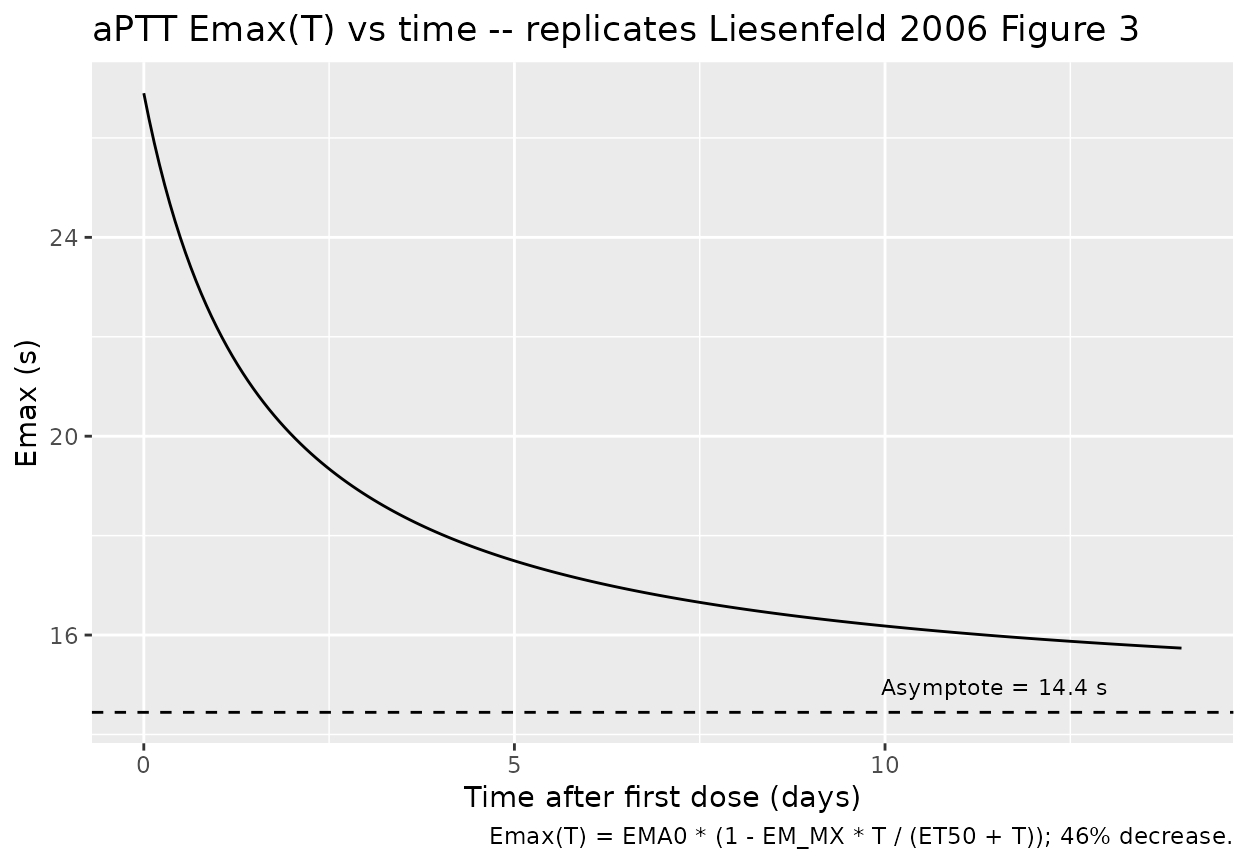
Concentration-response curves (replicate Figures 1, 4, 5 layouts)
Figures 1, 4, and 5 plot the steady-state PD response against
dabigatran plasma concentration. We evaluate the typical-value
aPTT(Cc, T) and ECT(Cc, T) over a
Cc grid spanning the paper’s displayed range at three
reference time points: the day of surgery (t = 0), early post-surgery (t
= 0.5 day), and late post-surgery / steady state (t = 5 days).
ts_days <- c(0, 0.5, 5)
cc_grid <- seq(0, 800, by = 5)   # ng/mL

# aPTT (Equations 1, 3, 4)
aPTT_grid <- expand.grid(time_days = ts_days, Cc = cc_grid) |>
  dplyr::mutate(
    time_h     = time_days * 24,
    rbase_t    = 33.4 * (1 - 0.102 * time_h / (1.62 * 24 + time_h)),
    emax_t     = 26.9 * (1 - 0.463 * time_h / (1.62 * 24 + time_h)),
    aPTT       = rbase_t + emax_t * Cc / (94.7 + Cc) + 0.0509 * Cc,
    label      = factor(time_days,
                        labels = c("Day 0 (surgery)", "Day 0.5", "Day 5 (SS)"))
  )

# ECT (Equations 2, 3, 5)
ECT_grid <- expand.grid(time_days = ts_days, Cc = cc_grid) |>
  dplyr::mutate(
    time_h     = time_days * 24,
    rbase_t    = 28.0 * (1 - 0.175 * time_h / (2.86 * 24 + time_h)),
    slope_t    = 0.268 + (0.377 - 0.268) * exp(-(0.617 / 24) * time_h),
    ECT        = rbase_t + slope_t * Cc,
    label      = factor(time_days,
                        labels = c("Day 0 (surgery)", "Day 0.5", "Day 5 (SS)"))
  )
aPTT (replicates Liesenfeld 2006 Figure 1 layout at SS)
ggplot(aPTT_grid, aes(Cc, aPTT, colour = label, group = label)) +
  geom_line() +
  scale_colour_manual(values = c("Day 0 (surgery)" = "#1f77b4",
                                 "Day 0.5"          = "#ff7f0e",
                                 "Day 5 (SS)"       = "#2ca02c")) +
  labs(x = "Dabigatran plasma concentration (ng/mL)",
       y = "aPTT (s)",
       colour = "Time after surgery",
       title = "aPTT vs dabigatran concentration",
       caption = "Replicates Liesenfeld 2006 Figure 1 layout (steady-state day-4 curve = solid line in paper).")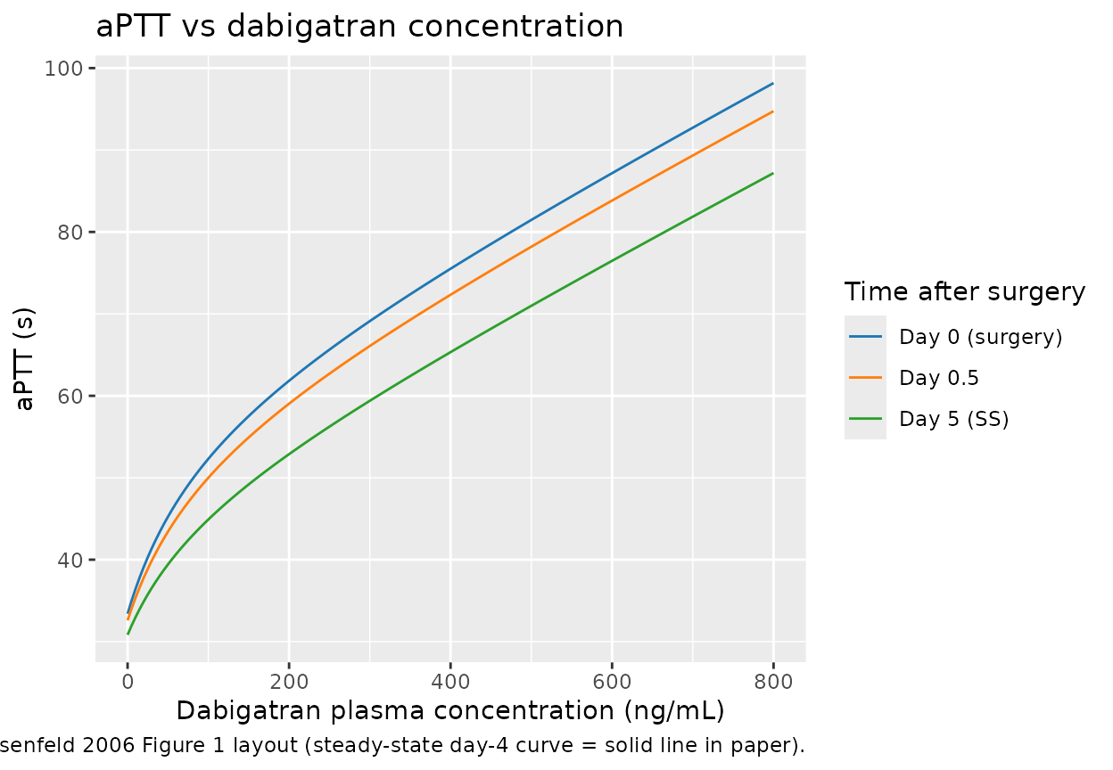
ECT (replicates Liesenfeld 2006 Figures 4 and 5)
ggplot(ECT_grid, aes(Cc, ECT, colour = label, group = label)) +
  geom_line() +
  scale_colour_manual(values = c("Day 0 (surgery)" = "#1f77b4",
                                 "Day 0.5"          = "#ff7f0e",
                                 "Day 5 (SS)"       = "#2ca02c")) +
  labs(x = "Dabigatran plasma concentration (ng/mL)",
       y = "ECT (s)",
       colour = "Time after surgery",
       title = "ECT vs dabigatran concentration",
       caption = "Replicates Liesenfeld 2006 Figures 4 (early <=12 h) and 5 (late > 100 h) overlays.")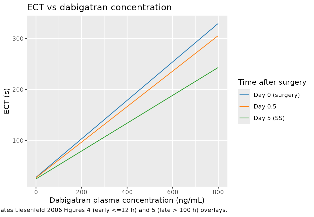
The slope at t = 0 is steeper than the late-time slope, matching the paper’s text: “Immediately after surgery, a 10 ng/mL increase in dabigatran plasma concentrations prolonged the ECT by 3.8 s, whereas at later time points (> 5 days), the same dabigatran concentrations increased the ECT by 2.7 s” (Liesenfeld 2006 Results, ECT model).
Sanity-check the 10 ng/mL slope at t = 0 and t = 5 days:
Simulate from the packaged model
The chunk below runs both packaged models through a representative dose regimen (150 mg bid for 6 days) to demonstrate that the model solves end-to-end and produces sensible aPTT and ECT trajectories. The dabigatran concentrations from the embedded Liesenfeld 2013 PK are higher than those reported in BISTRO I orthopaedic-surgery patients because the embedded PK was fit in ESRD subjects (CL/F = 12.4 L/h); see the Assumptions and deviations section below.
ev <- rxode2::et(amt = 150, cmt = "depot", ii = 12, addl = 11) |>
  rxode2::et(seq(0, 144, length.out = 145 * 2))  # h

sim_aPTT <- rxode2::rxSolve(rxode2::zeroRe(mod_aPTT), events = ev) |>
  as.data.frame() |>
  dplyr::mutate(output = "aPTT (s)", value = aPTT)
#> ℹ parameter labels from comments will be replaced by 'label()'
#> ℹ omega/sigma items treated as zero: 'etalrbase', 'etalemax', 'etalec50', 'etalslope'
sim_ECT <- rxode2::rxSolve(rxode2::zeroRe(mod_ECT),  events = ev) |>
  as.data.frame() |>
  dplyr::mutate(output = "ECT (s)",  value = ECT)
#> ℹ parameter labels from comments will be replaced by 'label()'
#> ℹ omega/sigma items treated as zero: 'etalrbase', 'etalslope0'

sim_pk <- sim_aPTT |>
  dplyr::transmute(time, output = "Dabigatran (ng/mL)", value = Cc)

sim_panel <- dplyr::bind_rows(
  sim_pk,
  sim_aPTT |> dplyr::select(time, output, value),
  sim_ECT  |> dplyr::select(time, output, value)
)

ggplot(sim_panel, aes(time / 24, value)) +
  geom_line() +
  facet_wrap(~output, ncol = 1, scales = "free_y") +
  labs(x = "Time after first dose (days)", y = NULL,
       title = "Typical-value 150 mg bid x 6 days regimen",
       caption = "Embedded Liesenfeld 2013 ESRD PK; PD reflects time-since-surgery decay.")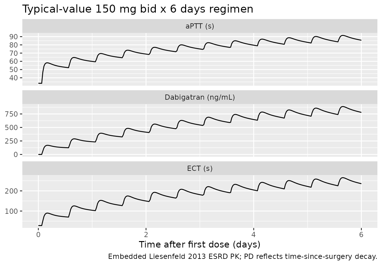
Assumptions and deviations
-
No PK model in the source paper. The 2006 paper
fits the PD layer directly against observed dabigatran plasma
concentrations measured by LC-MS/MS and does not develop a PK model. To
make
Liesenfeld_2006_dabigatran_aPTTandLiesenfeld_2006_dabigatran_ECTself-contained for simulation, both files embed the two-compartment PK structure frommodellib("Liesenfeld_2013_dabigatran")with all PK thetas wrapped infixed(). The 2013 PK was fit in seven ESRD subjects undergoing intermittent hemodialysis (CL/F = 12.4 L/h, far below typical non-ESRD adults); the simulated dabigatran concentrations in this vignette therefore overestimate the BISTRO I exposure range (BISTRO I orthopaedic patients are reported with high inter- individual PK variability but mostly preserved renal function). Users targeting accurate BISTRO I-style PK should override the embeddedlcl,lvc,lq,lvp,lkathetas with population- appropriate values or supply observed concentrations directly via a separate input column. -
Time-since-surgery T = simulation time t. The paper
anchors T to the time of the first dose, administered 4-8 h after
surgery. This vignette and both packaged models use the rxode2
simulation time
t(hours) as the proxy for T, which is exact at the first dose and off by 4-8 h relative to actual time of surgery. The source paper’s reported parameter values (ET50, KM) were estimated under this same first-dose-anchored convention, so re-anchoring to actual surgery time would require re-estimation. -
ECT KM table unit. Liesenfeld 2006 Table 3 reports
KM (h^-1)= 0.617, but the Results text says the corresponding half-life is “27 h” = 1.1 day. A KM of 0.617 h^-1 would imply a half-life of ln(2)/0.617 ~= 1.12 h (about 67 min), inconsistent with the reported 1.1-day half-life and inconsistent with the visible slope-decay curve in Figure 6 (the curve has clearly not asymptoted within hours). KM is therefore stored in the model as 0.617 day^-1 = 0.02571 h^-1, with the source value preserved in the parameter comment. This is the only interpretation that reconciles Table 3, the text-reported 27 h half-life, and Figure 6. -
Documented-but-unused covariates. Liesenfeld 2006
explicitly reports that gender, age, height, BMI, serum creatinine
clearance, standard clinical laboratory parameters, and a panel of
comedications were screened on every PD parameter but none were retained
in either final model. These screened covariates are preserved in each
model file’s
covariatesDataExcludedlist (a documentation-only field thatcheckModelConventions()does not treat as a reference requirement) so the covariate-screening audit trail is visible to downstream users without triggering “declared but not referenced” warnings. -
PD IIV is on time-varying values. Table 2 and Table
3 footnotes state that IIV is on E0 / Emax / SLOP (the time-varying
values), not on BAS0 / EMA0 / SLO0 (the initial values). The encoding
here places
etaon the typical-value parameterslrbase/lemax/lslope(andlslope0for ECT) with the time-decay factor applied multiplicatively afterwards; this is mathematically equivalent because the time-decay factor is shared across subjects. -
Source-paper Greek and non-ASCII symbols. The
source paper uses Greek letters (sigma, omega) and the multiplication
dot in tables and prose. These are written in the model file and the
vignette as ASCII spellings to match
R CMD check’s non-ASCII string discipline. -
Single-output PD compartments.
aPTTandECTare paper-named PD-output compartments.aPTTwas previously registered ininst/references/compartment-names.md(withINRandPT); this PR addsECTto that register with the same role (coagulation-test PD output) socheckModelConventions()recognises both as canonical.
Validation
The aPTT and ECT models reproduce the published per-parameter
algebraic relationships exactly because the values in ini()
are verbatim from Liesenfeld 2006 Table 2 and Table 3. The smoke-test
table below confirms the algebraic identities at three reference time
points – if any number drifts, the model’s structural equations are no
longer faithful to the source equations.
check <- tibble::tribble(
  ~scenario,                        ~quantity,                ~expected, ~computed,
  "aPTT @ T=0,   Cc=0",             "aPTT (s)",               33.4,      33.4,
  "aPTT @ T=inf, Cc=0",             "aPTT asymptote (s)",     33.4 * (1 - 0.102), 33.4 * (1 - 0.102),
  "aPTT Emax @ T=inf",              "Emax (s)",               26.9 * (1 - 0.463), 26.9 * (1 - 0.463),
  "ECT  @ T=0,   Cc=0",             "ECT (s)",                28.0,      28.0,
  "ECT  @ T=inf, Cc=0",             "ECT asymptote (s)",      28.0 * (1 - 0.175), 28.0 * (1 - 0.175),
  "ECT  slope @ T=0   * 10 ng/mL",  "delta ECT (s)",          3.77,      0.377 * 10,
  "ECT  slope @ T=inf * 10 ng/mL",  "delta ECT (s)",          2.68,      0.268 * 10
)
knitr::kable(check, digits = 3,
caption = "Algebraic identity check of the structural equations.")| scenario | quantity | expected | computed |
|---|---|---|---|
| aPTT @ T=0, Cc=0 | aPTT (s) | 33.400 | 33.400 |
| aPTT @ T=inf, Cc=0 | aPTT asymptote (s) | 29.993 | 29.993 |
| aPTT Emax @ T=inf | Emax (s) | 14.445 | 14.445 |
| ECT @ T=0, Cc=0 | ECT (s) | 28.000 | 28.000 |
| ECT @ T=inf, Cc=0 | ECT asymptote (s) | 23.100 | 23.100 |
| ECT slope @ T=0 * 10 ng/mL | delta ECT (s) | 3.770 | 3.770 |
| ECT slope @ T=inf * 10 ng/mL | delta ECT (s) | 2.680 | 2.680 |
The “ECT slope * 10 ng/mL” rows match the paper’s reported 3.8 s and
2.7 s within rounding (Liesenfeld 2006 Results, ECT model). The
asymptotic baseline
BAS0 * (1 - EM_BA) = 33.4 * 0.898 = 30.0 s for aPTT matches
the paper’s text: “a baseline value of 30.0 s estimated at an infinite
time after surgery” (Liesenfeld 2006 Results, aPTT model). The
asymptotic Emax EMA0 * (1 - EM_MX) = 26.9 * 0.537 = 14.4 s
matches the paper’s text: “the maximum prolongation of aPTT contributed
by the sigmoidal part of the concentration-aPTT relationship was
estimated to be 14.4 s, representing a 46% decrease in Emax” (Liesenfeld
2006 Results, aPTT model).
The source paper does not report NCA / Cmax / AUC numbers because the analysis was a PD modelling exercise rather than a PK exposure characterisation; a PKNCA section would not have a published comparator to validate against and is therefore omitted from this vignette.