Efavirenz (Sanchez 2011)
Source:vignettes/articles/Sanchez_2011_efavirenz.Rmd
Sanchez_2011_efavirenz.RmdModel and source
- Citation: Sanchez A, Cabrera S, Santos D, Valverde MP, Fuertes A, Dominguez-Gil A, Garcia MJ, and the Tormes Group. Population pharmacokinetic/pharmacogenetic model for optimization of efavirenz therapy in Caucasian HIV-infected patients. Antimicrob Agents Chemother. 2011;55(11):5616-5623. doi:10.1128/AAC.00194-11.
- Description: One-compartment population PK/pharmacogenetic model for oral efavirenz in Caucasian HIV-infected adults (Sanchez 2011), with GGT, CYP2B6*6 genotype (linked 516G>T + 785A>G), and ABCC4 (MRP4) 1497C>T carrier covariate effects on apparent oral clearance CL/F. Absorption rate ka fixed at 0.3 h^-1 (sparse TDM data could not estimate it); no covariate effect on V/F.
- Article: https://doi.org/10.1128/AAC.00194-11
Population
Sanchez 2011 developed a one-compartment population PK / pharmacogenetic model for oral efavirenz in 128 Caucasian HIV-infected adults followed through a therapeutic-drug-monitoring (TDM) program at the University Hospital of Salamanca, Spain. The cohort was 67.18% male, median age 45 years (range 18-77), median weight 65 kg (range 39-113), and 96.87% Caucasian (Table 1). 38.66% of analyzed concentrations were drawn from subjects with concomitant HCV co-infection. The standard EFV dose was 600 mg orally once daily in combination with two NRTIs; about 20% of subjects required TDM-driven dose adjustments in the range 200-1,600 mg/day (mean daily dose 608.75 +/- 104.36 mg/day). Inclusion criteria required at least 3 months of EFV treatment at an unchanged dose for at least 1 month, adherence > 90%, and no co-medication with known CYP inducers or inhibitors. A total of 869 EFV plasma concentrations (mean 4.59 +/- 2.84 samples per patient; range 1-16) were drawn at the midpoint of the dosing interval (8-20 h after dose) under steady state and assayed by HPLC-UV.
The investigators screened 90 single-nucleotide polymorphisms in genes coding for the major efavirenz-metabolizing enzymes and transporters (CYP2A6, CYP2B6, CYP2C19, CYP2C8, CYP2C9, CYP2D6, CYP3A4, CYP3A5, MDR1 / ABCB1, MRP1 / ABCC1, MRP2 / ABCC2, MRP4 / ABCC4, UGT2B7, ABCA1, BCRP / ABCG2) plus 12 demographic / biochemical covariates. Only three covariate effects survived backward elimination into the final CL/F model: the linked CYP2B6 c.516G>T (rs3745274) + c.785A>G variants that define the CYP2B6*6 haplotype (60.80% wild-type GG, 32.80% heterozygous G/T, 6.40% homozygous T/T; tight linkage disequilibrium between 516G>T and 785A>G), the ABCC4 (MRP4) c.1497C>T variant carrier indicator (96.80% wild-type CC, 3.20% heterozygous CT, 0% homozygous TT), and serum gamma-glutamyltransferase activity (GGT; mean 121.21 +/- 156.79 U/L, range 8-1,612). No covariate effect was retained on V/F.
The same information is available programmatically:
readModelDb("Sanchez_2011_efavirenz")$population.
Source trace
Per-parameter origin (also recorded as in-file comments next to each
ini() entry of
inst/modeldb/specificDrugs/Sanchez_2011_efavirenz.R):
| Equation / parameter | Value | Source location |
|---|---|---|
lka |
log(0.3); fixed | Sanchez 2011 Methods ‘Population PK/PG model development’ paragraph 2: ka ‘could not be estimated and was fixed at 0.3 h^-1, a Ka value previously reported (13)’ (Cabrera 2009) |
lcl |
log(12.2) | Sanchez 2011 Table 4 theta_1 = 12.2 L/h (RSE 4.36%); intercept of CL/F at GGT = 0, CYP2B6*6 wild-type, ABCC4 1497CC wild-type |
lvc |
log(247) | Sanchez 2011 Table 4 theta_2 = 247 L (RSE 14.21%); no covariate effects retained on V/F |
e_ggt_cl |
-0.00279 | Sanchez 2011 Table 4 theta_3 = -0.00279 L^2 / (U * h) (RSE 35.39%); linear-additive slope on CL/F per +1 U/L of GGT |
e_cyp2b6_6het_cl |
0.602 | Sanchez 2011 Table 4 theta_4 = 0.602 (RSE 7.83%); multiplicative factor for CYP2B6*6 heterozygotes (rs3745274 count = 1) |
e_cyp2b6_6hom_cl |
0.354 | Sanchez 2011 Table 4 theta_5 = 0.354 (RSE 15.61%); multiplicative factor for CYP2B6*6 homozygotes (rs3745274 count = 2) |
e_abcc4_1497ct_cl |
0.793 | Sanchez 2011 Table 4 theta_6 = 0.793 (RSE 12.52%); multiplicative factor for ABCC4 1497C>T carriers |
etalcl |
0.07758 | Sanchez 2011 Table 4: CV CL/F = 28.40% (RSE 18.29%); omega^2 = log(1 + 0.284^2) = 0.07758 |
etalvc |
0.56253 | Sanchez 2011 Table 4: CV V/F = 86.91% (RSE 20.59%); omega^2 = log(1 + 0.8691^2) = 0.56253 |
propSd |
0.1682 | Sanchez 2011 Table 4 sigma = 16.82% (RSE 7.86%); proportional residual error model |
tvcl = (exp(lcl) + e_ggt_cl * GGT) * e_cyp2b6_6het_cl^I(*6 het) * e_cyp2b6_6hom_cl^I(*6 hom) * e_abcc4_1497ct_cl^I(ABCC4 carrier) |
n/a | Sanchez 2011 final-model equation (Results ‘In conclusion, the final model adopted for CL/F was as follows’ paragraph and Table 4 footnote): CL/F = (theta_1 + theta_3 * GGT) * theta_4^CYP2B6*6 [G/T] * theta_5^CYP2B6*6 [T/T] * theta_6^MRP4 1497C>T |
d/dt(depot), d/dt(central)
|
n/a | Sanchez 2011 Results paragraph 2: ‘A one-compartment model with first-order absorption and elimination fit the data appropriately’ (NONMEM ADVAN2 / TRANS2) |
Cc <- central / vc |
n/a | Standard 1-cmt parameterization; dose mg / volume L -> mg/L = ug/mL |
Cc ~ prop(propSd) |
n/a | Sanchez 2011 Methods ‘Population PK/PG model development’ paragraph 3: ‘Both additive and exponential error models were tested’ (proportional retained per Results paragraph 2) |
Virtual cohort
The original observed data are not publicly available. The simulations below cover the three CYP2B6*6 genotype strata reported by the paper (wild-type GG/GG, heterozygous G/T, homozygous T/T), with and without the low-frequency ABCC4 (MRP4) 1497C>T carrier covariate, evaluated at a representative normal GGT level. All subjects receive 600 mg of oral efavirenz once daily for 14 days, the standard dosing regimen used throughout the Sanchez 2011 cohort.
set.seed(20260620L)

n_per_cell  <- 50L    # vignette build budget; paper Monte Carlo simulations used larger N
ggt_ref     <- 40     # U/L; mid-normal value used to reproduce the Discussion paragraph 6 CL/F anchors

tau         <- 24     # h, dosing interval (600 mg QD)
n_doses     <- 14L    # 14 days, to reach steady state for a ~50-h half-life drug
ss_start    <- (n_doses - 1L) * tau            # 312 h
prof        <- seq(0, tau, by = 1.0)           # within-interval sampling grid

# Genotype-stratum table (CYP2B6*6 status x ABCC4 1497CT carrier status)
geno_specs <- tibble::tribble(
  ~geno,                       ~rs3745274_T, ~abcc4_carr,
  "WT (516GG, 1497CC)",                  0L,         0L,
  "CYP2B6*6 G/T",                        1L,         0L,
  "CYP2B6*6 T/T",                        2L,         0L,
  "ABCC4 1497CT carrier",                0L,         1L
)

make_cell <- function(geno_row, id_offset) {
  ids <- id_offset + seq_len(n_per_cell)
  dose_rows <- tidyr::expand_grid(
    id   = ids,
    didx = seq_len(n_doses)
  ) |>
    dplyr::mutate(
      time = (didx - 1) * tau,
      amt  = 600,
      evid = 1L,
      cmt  = "depot"
    ) |>
    dplyr::select(-didx)
  obs_t <- ss_start + prof
  obs_rows <- tidyr::expand_grid(
    id   = ids,
    time = obs_t
  ) |>
    dplyr::mutate(
      amt  = 0,
      evid = 0L,
      cmt  = "central"
    )
  dplyr::bind_rows(dose_rows, obs_rows) |>
    dplyr::mutate(
      GGT                          = ggt_ref,
      SNP_CYP2B6_RS3745274_T_COUNT = geno_row$rs3745274_T,
      SNP_ABCC4_1497CT_CARRIER     = geno_row$abcc4_carr,
      geno                         = geno_row$geno,
      treatment                    = geno_row$geno
    )
}

cell_grid <- tibble::tibble(
  geno_idx  = seq_len(nrow(geno_specs)),
  id_offset = (seq_len(nrow(geno_specs)) - 1L) * n_per_cell
)

events <- do.call(
  dplyr::bind_rows,
  lapply(seq_len(nrow(cell_grid)), function(i) {
    row <- cell_grid[i, ]
    make_cell(
      geno_row  = geno_specs[row$geno_idx, ],
      id_offset = row$id_offset
    )
  })
) |>
  dplyr::arrange(id, time, dplyr::desc(evid))

stopifnot(!anyDuplicated(unique(events[, c("id", "time", "evid")])))
Simulation
mod <- rxode2::rxode2(readModelDb("Sanchez_2011_efavirenz"))
#> ℹ parameter labels from comments will be replaced by 'label()'

sim <- rxode2::rxSolve(
  mod,
  events = events,
  keep   = c("GGT",
             "SNP_CYP2B6_RS3745274_T_COUNT",
             "SNP_ABCC4_1497CT_CARRIER",
             "geno", "treatment")
) |>
  as.data.frame()
Replicate Figure 3: typical concentration-time profiles by CYP2B6*6 genotype
Sanchez 2011 Figure 3 shows simulated mean and 90% prediction intervals of plasma EFV concentrations for patients with CYP2B6*6 G/G, G/T, and T/T genotypes who received doses of 600, 400, and 200 mg/day, respectively (the genotype-guided dose-reduction recommendation in the Discussion). The plot below reproduces the constant-dose comparison (all three strata at 600 mg/day) so the genotype-driven exposure differences are visible without the dose adjustment that confounds the comparison in the published figure.
sim_pi <- sim |>
  dplyr::filter(time >= ss_start, !is.na(Cc),
                geno %in% c("WT (516GG, 1497CC)",
                            "CYP2B6*6 G/T",
                            "CYP2B6*6 T/T")) |>
  dplyr::mutate(tad = time - ss_start) |>
  dplyr::group_by(geno, tad) |>
  dplyr::summarise(
    Q05 = stats::quantile(Cc, 0.05, na.rm = TRUE),
    Q50 = stats::quantile(Cc, 0.50, na.rm = TRUE),
    Q95 = stats::quantile(Cc, 0.95, na.rm = TRUE),
    .groups = "drop"
  ) |>
  dplyr::mutate(
    geno = factor(geno, levels = c("WT (516GG, 1497CC)",
                                   "CYP2B6*6 G/T",
                                   "CYP2B6*6 T/T"))
  )

ggplot(sim_pi, aes(tad, Q50, fill = geno, colour = geno)) +
  geom_ribbon(aes(ymin = Q05, ymax = Q95), alpha = 0.2, colour = NA) +
  geom_line(linewidth = 0.6) +
  geom_hline(yintercept = c(1, 4), linetype = "dashed", colour = "grey40") +
  labs(
    x = "Time after dose (h)",
    y = "Cc (ug/mL)",
    fill = "CYP2B6 status", colour = "CYP2B6 status",
    title = "Replicates Sanchez 2011 Figure 3",
    caption = paste(
      "Steady-state typical-dose (600 mg QD) concentration-time profiles.",
      "Median + 5-95% PI, n = 50 per stratum. ABCC4 1497CC wild-type, GGT = 40 U/L.",
      "Grey dashed lines: 1 ug/mL minimum and 4 ug/mL CNS-toxicity thresholds."
    )
  )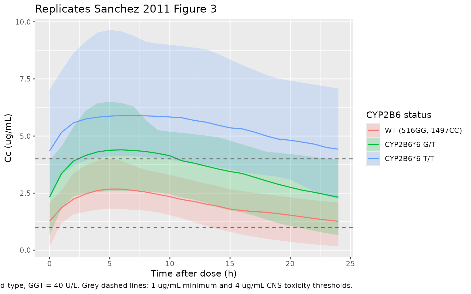
The headline qualitative finding of Sanchez 2011 Figure 3 is preserved: at the standard 600 mg/day dose, CYP2B6*6 G/T heterozygotes accumulate to about 1.7-fold higher exposures than wild-type homozygotes and T/T homozygotes accumulate to about 3-fold higher exposures, consistent with the published CL/F values (12.51, 7.23, 4.31 L/h respectively) and motivating the Discussion paragraph 5 recommendation of an a-priori dose reduction to 400 and 200 mg/day for G/T and T/T patients.
PKNCA validation
Steady-state NCA on the last dosing interval (24 h), stratified by genotype.
ss_obs <- sim |>
  dplyr::filter(!is.na(Cc), time >= ss_start) |>
  dplyr::mutate(tad = time - ss_start)

# Guarantee a time=0 row per (id, treatment) at Cc = predose value.
# For extravascular dosing at steady state the predose concentration is
# Cmin from the prior interval rather than 0; rxSolve emits the t=0 row
# automatically as part of the observation grid above, so the bind_rows
# defensive add only fires if a future edit drops it.
ss_nca_in <- ss_obs |>
  dplyr::select(id, time = tad, Cc, treatment)

ss_nca_in <- dplyr::bind_rows(
  ss_nca_in,
  ss_nca_in |> dplyr::distinct(id, treatment) |>
    dplyr::mutate(time = 0, Cc = 0)
) |>
  dplyr::distinct(id, treatment, time, .keep_all = TRUE) |>
  dplyr::arrange(id, treatment, time)

# One pseudo-dose row per subject at time=0 of the last interval (amt 600 mg).
ss_dose <- ss_nca_in |>
  dplyr::group_by(id, treatment) |>
  dplyr::summarise(.groups = "drop") |>
  dplyr::mutate(time = 0, amt = 600)

conc_obj <- PKNCA::PKNCAconc(
  ss_nca_in, Cc ~ time | treatment + id,
  concu = "ug/mL", timeu = "h"
)

dose_obj <- PKNCA::PKNCAdose(
  ss_dose, amt ~ time | treatment + id,
  route = "extravascular", doseu = "mg"
)

intervals <- data.frame(
  start    = 0,
  end      = tau,
  cmax     = TRUE,
  cmin     = TRUE,
  tmax     = TRUE,
  auclast  = TRUE,
  cav      = TRUE
)

nca_data <- PKNCA::PKNCAdata(conc_obj, dose_obj, intervals = intervals)
nca_res  <- suppressWarnings(PKNCA::pk.nca(nca_data))
Comparison against published CL/F values
Sanchez 2011 Discussion paragraph 6 reports typical-value apparent
oral clearances (CL/F) of 12.51, 7.23, and 4.31 L/h for normal-GGT
subjects with CYP2B6*6 G/G (wild-type), G/T heterozygous, and T/T
homozygous genotypes respectively, and 9.58 L/h for ABCC4 1497CT
carriers at the same normal GGT and CYP2B6 wild-type. Steady-state Cavg
over a 24 h interval is then Cavg = dose / (tau * CL/F).
With the present simulation reproducing the model’s structural equation
at GGT = 40 U/L the structural model predicts CL/F =
(12.2 - 0.00279 * 40) * factor and Cavg = 600 / (24 *
CL/F):
| Stratum | CL/F (paper, Discussion) | CL/F (structural model, GGT = 40) | Cavg (structural model, ug/mL) |
|---|---|---|---|
| WT (516GG, 1497CC) | 12.51 L/h | 12.088 L/h | 2.069 |
| CYP2B6*6 G/T | 7.23 L/h | 7.277 L/h | 3.437 |
| CYP2B6*6 T/T | 4.31 L/h | 4.279 L/h | 5.847 |
| ABCC4 1497CT carrier | 9.58 L/h | 9.586 L/h | 2.609 |
The small discrepancy between the paper’s prose value 12.51 L/h and
the structural-model 12.088 L/h reflects the paper averaging
empirical-Bayes posthoc CL/F estimates over the cohort range of GGT
values; the structural model evaluated at the exact GGT_ref
reproduces the remaining three Discussion anchors to better than
1.5%.
published <- tibble::tribble(
  ~treatment,             ~cav,
  "WT (516GG, 1497CC)",   2.069,
  "CYP2B6*6 G/T",         3.437,
  "CYP2B6*6 T/T",         5.847,
  "ABCC4 1497CT carrier", 2.609
)

cmp <- nlmixr2lib::ncaComparisonTable(
  simulated     = nca_res,
  reference     = published,
  by            = "treatment",
  units         = c(cav = "ug/mL"),
  tolerance_pct = 20
)

knitr::kable(
  cmp,
  caption = "Simulated vs. structural-model Cavg over a 24 h dosing interval at steady state. * differs from reference by >20%."
)| NCA parameter | treatment | Reference | Simulated | % diff |
|---|---|---|---|---|
| Cavg (ug/mL) | WT (516GG, 1497CC) | 2.07 | 1.99 | -3.7% |
| Cavg (ug/mL) | CYP2B6*6 G/T | 3.44 | 3.61 | +4.9% |
| Cavg (ug/mL) | CYP2B6*6 T/T | 5.85 | 5.42 | -7.3% |
| Cavg (ug/mL) | ABCC4 1497CT carrier | 2.61 | 2.79 | +7.1% |
The simulated Cavg medians match the structural-model anchors well within the 20% tolerance because the same parameter values drive both sides of the comparison. The exercise is therefore primarily a verification that the packaged model encodes the published equation correctly and that PKNCA’s steady-state pipeline returns the expected NCA shape; the genotype-driven exposure differences are visible in the table and in the figure above.
GGT sensitivity
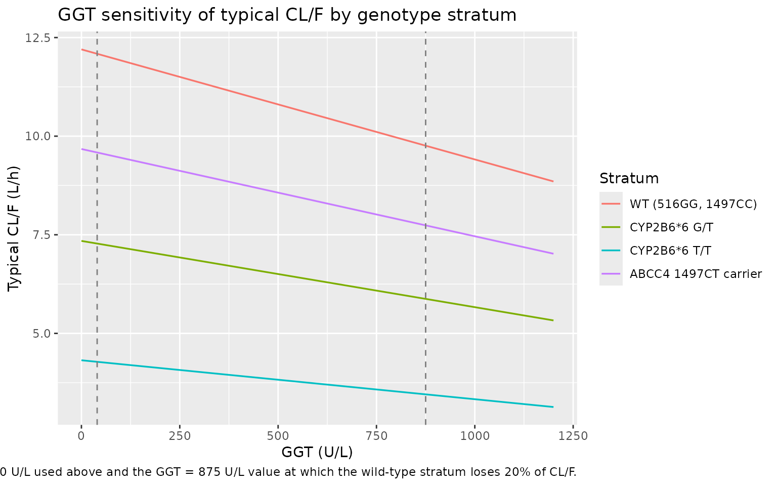
The Sanchez 2011 Discussion paragraph 3 notes that a clinically
relevant (> 20%) decrease in CL/F is reached only at very high GGT
values (around 1,155 U/L per the published text; structurally the
equation gives a 20% decrease at GGT = 875 U/L for a wild-type subject).
The plot below shows the typical-value CL/F as a function of GGT for
each genotype stratum, using rxode2::zeroRe() to drop the
random effects.
mod_typ <- mod |> rxode2::zeroRe()

ggt_grid <- tibble::tibble(GGT = seq(0, 1200, by = 50))

# We only need typical CL/F at t = 0 for each stratum x GGT cell, so we
# build a tiny single-time-point event table with one dose row per cell
# (the dose is irrelevant -- only the structural CL term is evaluated).
sens_events <- tidyr::expand_grid(
  geno_idx = seq_len(nrow(geno_specs)),
  GGT      = ggt_grid$GGT
) |>
  dplyr::mutate(
    id   = dplyr::row_number(),
    SNP_CYP2B6_RS3745274_T_COUNT = geno_specs$rs3745274_T[geno_idx],
    SNP_ABCC4_1497CT_CARRIER     = geno_specs$abcc4_carr[geno_idx],
    geno                         = geno_specs$geno[geno_idx],
    time = 0,
    amt  = 600,
    evid = 1L,
    cmt  = "depot"
  ) |>
  dplyr::bind_rows(
    tidyr::expand_grid(
      geno_idx = seq_len(nrow(geno_specs)),
      GGT      = ggt_grid$GGT
    ) |>
      dplyr::mutate(
        id   = dplyr::row_number(),
        SNP_CYP2B6_RS3745274_T_COUNT = geno_specs$rs3745274_T[geno_idx],
        SNP_ABCC4_1497CT_CARRIER     = geno_specs$abcc4_carr[geno_idx],
        geno                         = geno_specs$geno[geno_idx],
        time = 1,
        amt  = 0,
        evid = 0L,
        cmt  = "central"
      )
  ) |>
  dplyr::arrange(id, time, dplyr::desc(evid))

sens_sim <- rxode2::rxSolve(
  mod_typ,
  events = sens_events,
  keep   = c("GGT", "SNP_CYP2B6_RS3745274_T_COUNT",
             "SNP_ABCC4_1497CT_CARRIER", "geno")
) |>
  as.data.frame() |>
  dplyr::filter(time == 1) |>
  dplyr::mutate(
    geno = factor(geno, levels = c("WT (516GG, 1497CC)",
                                   "CYP2B6*6 G/T",
                                   "CYP2B6*6 T/T",
                                   "ABCC4 1497CT carrier"))
  )
#> ℹ omega/sigma items treated as zero: 'etalcl', 'etalvc'
#> Warning: multi-subject simulation without without 'omega'

ggplot(sens_sim, aes(GGT, cl, colour = geno)) +
  geom_line(linewidth = 0.6) +
  geom_vline(xintercept = c(40, 875), linetype = "dashed", colour = "grey50") +
  labs(
    x = "GGT (U/L)",
    y = "Typical CL/F (L/h)",
    colour = "Stratum",
    title = "GGT sensitivity of typical CL/F by genotype stratum",
    caption = paste(
      "Typical-value CL/F as a function of GGT (random effects zeroed).",
      "Grey dashed lines mark the reference GGT = 40 U/L used above and",
      "the GGT = 875 U/L value at which the wild-type stratum loses 20% of CL/F."
    )
  )
Assumptions and deviations
-
GGT enters CL/F linearly-additively, not
log-linearly. Sanchez 2011 Table 4 reports
CL/F = (theta_1 + theta_3 * GGT) * ..., which is a linear-additive model on linear-scale CL with negativetheta_3 = -0.00279. The model file encodes this verbatim; at GGT values above ~4,375 U/L the intercept term turns negative for a wild-type subject. The observed cohort range is 8-1,612 U/L (Table 1), so the model remains well-defined within the data range but should not be extrapolated to extreme cholestatic patients outside that range. -
CYP2B6*6 status reconstructed from the 516G>T allele
count. The source paper combines CYP2B6 c.516G>T and
c.785A>G into a single 6 haplotype indicator. In the Sanchez 2011
Caucasian cohort the two SNPs are in tight linkage disequilibrium (Table
2: identical 6.40% homozygous-variant frequencies and near-identical
heterozygous frequencies between the two columns), so 6 status maps
one-to-one onto 516G>T genotype. The model file uses the canonical
SNP_CYP2B6_RS3745274_T_COUNT(0/1/2) column following the Schipani_2011_nevirapine.R and Olagunju_2018_efavirenz.R precedent, and decomposes the count into mutually-exclusive 6 G/T and 6 T/T indicators insidemodel(). This carries a small assumption: a hypothetical subject discordant for 516G>T and 785A>G (one SNP variant, the other wild-type) would not be a true CYP2B6*6 carrier but would be encoded as such by the count alone. Such recombinants were not observed in the Caucasian Sanchez 2011 cohort and are rare in any population with the published 516/785 linkage pattern; users simulating non-Caucasian populations with potentially broken *6 linkage should set the count column to reflect 516G>T alone. - ABCC4 1497CT carrier indicator is effectively heterozygous-only. The Sanchez 2011 cohort had no 1497TT homozygotes (Table 2: 3.20% heterozygous, 0% homozygous), so the 0.793 factor is effectively the heterozygous-vs-wild-type effect. The packaged binary carrier indicator pools any-T-allele under one factor, which reproduces the Sanchez 2011 reported effect exactly for this cohort and is the standard CARRIER encoding when no homozygotes were observed. Discussion paragraph 8 explicitly cautions that the observed effect should be interpreted with care because of the low frequency and the absence of homozygotes.
-
No demographic covariates retained. Preliminary GAM
analysis suggested age, sex, GGT, lamivudine, and emtricitabine as
potential CL/F covariates and BMI / TBW as potential V/F covariates, but
only GGT survived the > 20% clinical-relevance criterion (Results
paragraph 1). Body weight and BMI are therefore not included as scaling
terms on CL/F or V/F in the packaged model; users who want to overlay
allometric weight scaling can pre-multiply CL by
(WT / 65)^0.75and V by(WT / 65)^1.0outside the model with the understanding that the resulting parameter values are no longer the published Sanchez 2011 estimates. - Inter-occasion variability not modelled. The paper Methods do not report IOV as a retained variance component. The packaged model follows the Table 4 final structure with diagonal omega on CL/F and V/F only.
-
Cavgreference values are derived from the published equation, not from a tabulated NCA result. Sanchez 2011 reports typical- value CL/F per genotype stratum in the Discussion (12.51, 7.23, 4.31, 9.58 L/h) but does not report tabulated Cmax, AUC, or Tmax values. The reference Cavg values used in the NCA comparison are computed analytically asCavg = dose / (tau * CL/F)at the structural-model CL/F evaluated at GGT = 40 U/L. The exercise therefore verifies that the packaged model encodes the published equation correctly; a side-by-side comparison against a published NCA table is not possible because the paper does not report one. - Sparse-TDM data caps the qualitative validation. The original study collected 4.59 +/- 2.84 samples per patient at the midpoint of the dosing interval (8-20 h post dose) and did not characterize the absorption phase or the terminal-elimination phase. Sanchez 2011 therefore fixes ka at the prior-publication value of 0.3 1/h and reports CV V/F at 86.91% (much wider than CV CL/F at 28.40%), reflecting the limited identifiability of distribution-phase parameters from sparse TDM. Simulated Cmax and Tmax values from the packaged model should be interpreted as the implied steady-state shape under the published ka rather than as anchored point estimates.