Model and source
- Citation: Li TY, Liu X, Tang L, Cai W, Zhang J, Su Y, Yu C, Liu BJ, Jiang LF, Liu C, Yu YX. Dose Optimization of Rivaroxaban in Elderly Chinese Patients with Non-Valvular Atrial Fibrillation: Analysis of Populations Pharmacokinetics and Exposure-Response Relationships. Drug Des Devel Ther. 2025;19:10703. doi:10.2147/DDDT.S563521.
- Description: One-compartment population PK model for oral rivaroxaban in elderly (65 years and older) Chinese patients with non-valvular atrial fibrillation, with a creatinine-clearance power effect and a concomitant-amiodarone effect on CL/F (Li 2025)
- Article: https://doi.org/10.2147/DDDT.S563521 (open access, PMC12683255)
The article has no supplementary material. Every value in the model is printed in the main-text Table 2 and its footnote equation.
Population
Li 2025 fitted 256 rivaroxaban plasma concentrations from 93 Chinese patients aged 65 years and older with non-valvular atrial fibrillation (NVAF), enrolled prospectively at Suzhou Municipal Hospital (Nanjing Medical University) between January 2021 and March 2022. Patients had taken rivaroxaban 10, 15 or 20 mg once daily for at least 4 weeks; the dose was chosen by the treating clinician. Patients with CrCL < 15 mL/min, Child-Pugh B or C hepatic impairment, other anticoagulants, or a strong CYP3A4 / P-gp inhibitor were excluded (Methods “Study Design”).
The cohort is old and renally impaired: mean age 79 +/- 7 years (range 66-94), mean weight 61.4 +/- 12.1 kg, 50 men and 43 women, and a median Cockcroft-Gault creatinine clearance of 48.6 mL/min (range 14.3-91.7) with 73.1% below 50 mL/min. Amiodarone, usually 200 mg once daily for rhythm control, was the most common comedication (45 patients, 48.4%) (Table 1, Results “Population Characteristics”). At steady state each patient gave a trough sample 0.5 h before the next dose and a peak sample 3 +/- 1 h after a dose (Methods “Rivaroxaban Quantification”).
The same information is available programmatically via
readModelDb("Li_2025_rivaroxaban")()$population.
Source trace
| Equation / parameter | Value | Source location |
|---|---|---|
| One compartment, first-order absorption and elimination | n/a | Results “PopPK Model of Rivaroxaban” |
lka (fixed) |
log(0.821) |
Table 2 tvKa 0.821, fixed; Results “fixed to the
reported value (0.821 h-1)” |
lcl |
log(4.501) |
Table 2 final model tvCL (L/h) 4.501 (2.84)
|
lvc |
log(30.714) |
Table 2 final model tvV(L) 30.714 (2.19)
|
e_crcl_cl |
0.179 |
Table 2 final model dCLdCrCL 0.179 (18.61)
|
e_conmed_amio_cl |
-0.124 |
Table 2 final model dCLamiodarone -0.124 (30.51)
|
| CrCL reference 47.4 mL/min | 47.4 |
Table 2 footnote:
CL (L/h) = 4.5 * (CrCL/47.4)^0.18 * exp(amiodarone * -0.12)*exp(etaCL)
|
etalcl |
0.036 |
Table 2 final model omega2 CL (%) 3.6 [21]
|
etalvc |
0.033 |
Table 2 final model omega2 V (%) 3.3 [19]
|
addSd |
18.025 ng/mL |
Table 2 final model stdev0 18.025 (7.54); additive
residual model named in Results |
The footnote equation fixes both covariate forms: a power function of
CrCL / 47.4 and an exponential shift for amiodarone. The
footnote prints rounded values (4.5, 0.18, -0.12); the model uses the
three-decimal Table 2 estimates. The Discussion confirms both effects
arithmetically: “CL increased by approximately 1.8% for every 10%
elevation in CrCL” (1.1^0.179 = 1.017) and “reduction in CL
to 0.88-fold with concomitant amiodarone use”
(exp(-0.124) = 0.883).
Replicate published figures
Figures 3 and 4: steady-state AUC by renal function and amiodarone
Li 2025 simulated 10, 15 and 20 mg once daily in virtual patients
stratified by five CrCL bands and by amiodarone use, and summarised the
steady-state AUC24,ss as boxplots (Figure 3) and as the
probability that AUC24,ss lies in the typical NVAF range
1860-5434 ng*h/mL (Figure 4). At steady state,
AUC24,ss = Dose / (CL/F) exactly, so each virtual patient’s
clearance is all that is needed; the PKNCA section below confirms that
identity on full profiles.
set.seed(20251203)

n_per_cell <- 200L
bands <- tibble::tribble(
  ~band,    ~lo, ~hi,
  "15-29",   15,  29,
  "30-49",   30,  49,
  "50-69",   50,  69,
  "70-89",   70,  89,
  "90-110",  90, 110
)

grid <- tidyr::expand_grid(bands, CONMED_AMIO = c(0L, 1L)) |>
  mutate(cell = row_number())

cohort_f3 <- grid |>
  tidyr::uncount(n_per_cell) |>
  mutate(
    id = row_number(),
    # The paper does not say how CrCL was distributed inside each band; a
    # uniform draw across the band is used here.
    CRCL = stats::runif(n(), lo, hi)
  )

ev_f3 <- bind_rows(
  cohort_f3 |> transmute(id, time = 0, evid = 1L, amt = 10, cmt = "depot", CRCL, CONMED_AMIO),
  cohort_f3 |> transmute(id, time = 1, evid = 0L, amt = NA_real_, cmt = "central", CRCL, CONMED_AMIO)
) |>
  arrange(id, time, desc(evid))

mod <- readModelDb("Li_2025_rivaroxaban")

rxode2::rxSetSeed(20251203)
sim_f3 <- rxode2::rxSolve(mod, events = ev_f3) |> as.data.frame()
#> ℹ parameter labels from comments will be replaced by 'label()'

auc_f3 <- sim_f3 |>
  distinct(id, cl) |>
  left_join(cohort_f3 |> select(id, band, CONMED_AMIO), by = "id") |>
  tidyr::expand_grid(dose = c(10, 15, 20)) |>
  mutate(
    auc = 1000 * dose / cl,
    amio = ifelse(CONMED_AMIO == 1L, "With amiodarone", "Without amiodarone"),
    amio = factor(amio, levels = c("Without amiodarone", "With amiodarone")),
    band = factor(band, levels = bands$band)
  )

stopifnot(nrow(auc_f3) == 3L * nrow(cohort_f3))
# Replicates Figure 3 of Li 2025.
ggplot(auc_f3, aes(band, auc)) +
  geom_boxplot(outlier.shape = NA, fill = "#F4A582") +
  geom_hline(yintercept = c(1860, 5434), linetype = "dashed", colour = "red") +
  facet_grid(paste(dose, "mg QD") ~ amio) +
  coord_cartesian(ylim = c(0, 10500)) +
  labs(
    x = "CrCL (mL/min)",
    y = "AUC24,ss (ng*h/mL)",
    caption = paste(
      "Replicates Figure 3 of Li 2025. Dashed lines: typical NVAF AUC24,ss",
      "range 1860-5434 ng*h/mL."
    )
  )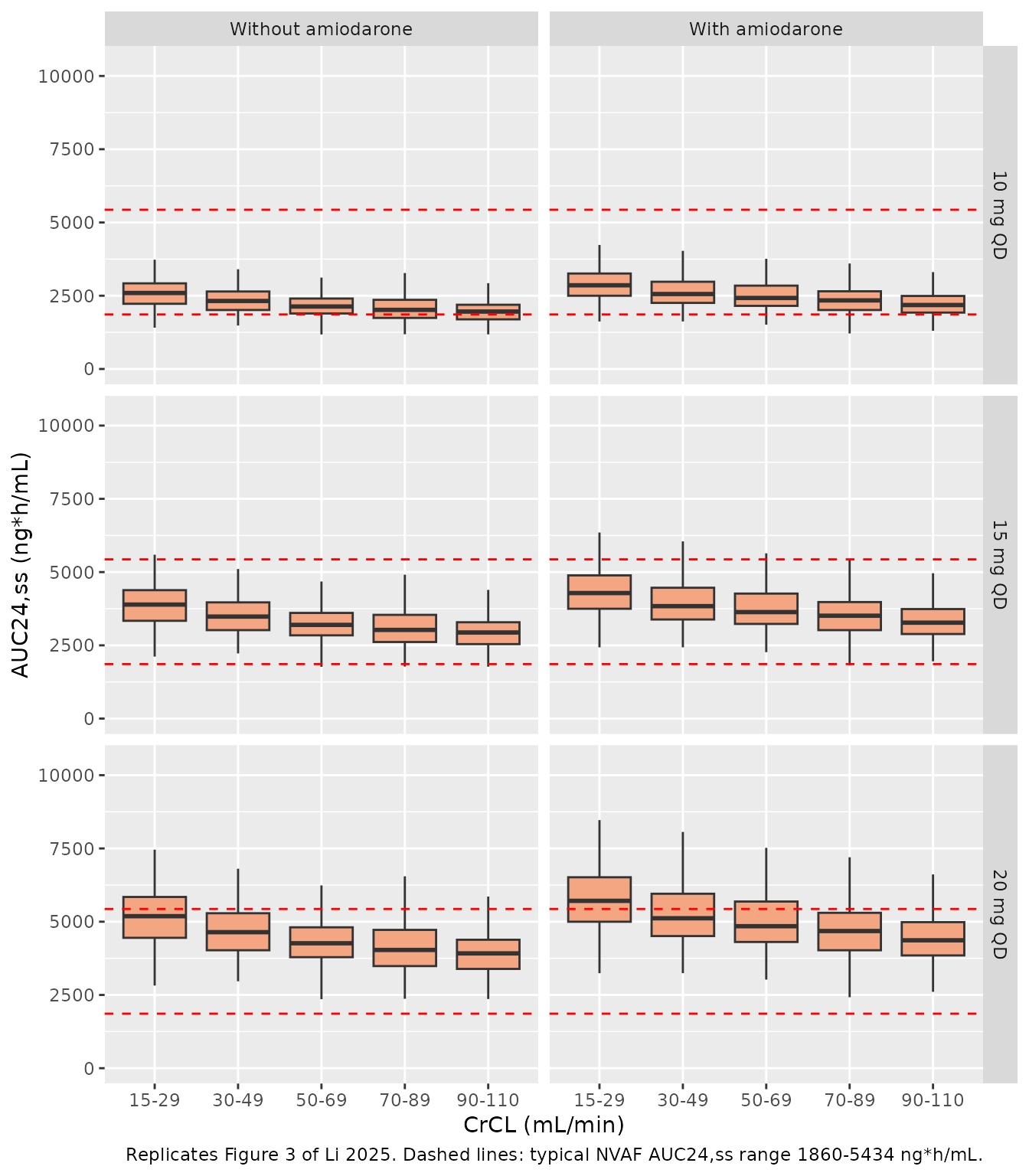
The medians below were digitised by the maintainers from Figure 3 (read to roughly +/- 50 ng*h/mL).
fig3_pub <- tibble::tribble(
  ~dose, ~amio,                ~band,    ~pub_median,
  10,    "Without amiodarone", "15-29",  2650,
  10,    "Without amiodarone", "30-49",  2330,
  10,    "Without amiodarone", "50-69",  2150,
  10,    "Without amiodarone", "70-89",  2000,
  10,    "Without amiodarone", "90-110", 1950,
  10,    "With amiodarone",    "15-29",  2830,
  10,    "With amiodarone",    "30-49",  2530,
  10,    "With amiodarone",    "50-69",  2430,
  10,    "With amiodarone",    "70-89",  2330,
  10,    "With amiodarone",    "90-110", 2290,
  15,    "Without amiodarone", "15-29",  3950,
  15,    "Without amiodarone", "30-49",  3480,
  15,    "Without amiodarone", "50-69",  3200,
  15,    "Without amiodarone", "70-89",  3030,
  15,    "Without amiodarone", "90-110", 2920,
  15,    "With amiodarone",    "15-29",  4230,
  15,    "With amiodarone",    "30-49",  3800,
  15,    "With amiodarone",    "50-69",  3620,
  15,    "With amiodarone",    "70-89",  3480,
  15,    "With amiodarone",    "90-110", 3420,
  20,    "Without amiodarone", "15-29",  5270,
  20,    "Without amiodarone", "30-49",  4640,
  20,    "Without amiodarone", "50-69",  4250,
  20,    "Without amiodarone", "70-89",  4040,
  20,    "Without amiodarone", "90-110", 3900,
  20,    "With amiodarone",    "15-29",  5650,
  20,    "With amiodarone",    "30-49",  5050,
  20,    "With amiodarone",    "50-69",  4830,
  20,    "With amiodarone",    "70-89",  4650,
  20,    "With amiodarone",    "90-110", 4570
)

f3_sim <- auc_f3 |>
  group_by(dose, amio, band) |>
  summarise(
    sim_median = median(auc),
    iqr_ratio = quantile(auc, 0.75) / quantile(auc, 0.25),
    pta = 100 * mean(auc >= 1860 & auc <= 5434),
    .groups = "drop"
  ) |>
  mutate(amio = as.character(amio), band = as.character(band))

f3_chk <- fig3_pub |>
  left_join(f3_sim, by = c("dose", "amio", "band")) |>
  mutate(pct_diff = 100 * (sim_median / pub_median - 1))

f3_chk |>
  select(dose, amio, band, pub_median, sim_median, pct_diff, iqr_ratio) |>
  rename(
    "Dose (mg)" = dose,
    "Amiodarone" = amio,
    "CrCL band (mL/min)" = band,
    "Figure 3 median" = pub_median,
    "Simulated median" = sim_median,
    "Difference (%)" = pct_diff,
    "Simulated Q3/Q1" = iqr_ratio
  ) |>
knitr::kable(digits = c(0, 0, 0, 0, 0, 1, 2), caption = "Median AUC24,ss (ng*h/mL), simulated versus Figure 3 of Li 2025.")| Dose (mg) | Amiodarone | CrCL band (mL/min) | Figure 3 median | Simulated median | Difference (%) | Simulated Q3/Q1 |
|---|---|---|---|---|---|---|
| 10 | Without amiodarone | 15-29 | 2650 | 2594 | -2.1 | 1.31 |
| 10 | Without amiodarone | 30-49 | 2330 | 2321 | -0.4 | 1.31 |
| 10 | Without amiodarone | 50-69 | 2150 | 2132 | -0.8 | 1.27 |
| 10 | Without amiodarone | 70-89 | 2000 | 2018 | 0.9 | 1.35 |
| 10 | Without amiodarone | 90-110 | 1950 | 1959 | 0.5 | 1.29 |
| 10 | With amiodarone | 15-29 | 2830 | 2856 | 0.9 | 1.30 |
| 10 | With amiodarone | 30-49 | 2530 | 2559 | 1.1 | 1.32 |
| 10 | With amiodarone | 50-69 | 2430 | 2423 | -0.3 | 1.32 |
| 10 | With amiodarone | 70-89 | 2330 | 2340 | 0.4 | 1.32 |
| 10 | With amiodarone | 90-110 | 2290 | 2183 | -4.7 | 1.30 |
| 15 | Without amiodarone | 15-29 | 3950 | 3891 | -1.5 | 1.31 |
| 15 | Without amiodarone | 30-49 | 3480 | 3482 | 0.0 | 1.31 |
| 15 | Without amiodarone | 50-69 | 3200 | 3198 | -0.1 | 1.27 |
| 15 | Without amiodarone | 70-89 | 3030 | 3027 | -0.1 | 1.35 |
| 15 | Without amiodarone | 90-110 | 2920 | 2939 | 0.7 | 1.29 |
| 15 | With amiodarone | 15-29 | 4230 | 4284 | 1.3 | 1.30 |
| 15 | With amiodarone | 30-49 | 3800 | 3838 | 1.0 | 1.32 |
| 15 | With amiodarone | 50-69 | 3620 | 3635 | 0.4 | 1.32 |
| 15 | With amiodarone | 70-89 | 3480 | 3511 | 0.9 | 1.32 |
| 15 | With amiodarone | 90-110 | 3420 | 3274 | -4.3 | 1.30 |
| 20 | Without amiodarone | 15-29 | 5270 | 5188 | -1.6 | 1.31 |
| 20 | Without amiodarone | 30-49 | 4640 | 4642 | 0.0 | 1.31 |
| 20 | Without amiodarone | 50-69 | 4250 | 4264 | 0.3 | 1.27 |
| 20 | Without amiodarone | 70-89 | 4040 | 4036 | -0.1 | 1.35 |
| 20 | Without amiodarone | 90-110 | 3900 | 3919 | 0.5 | 1.29 |
| 20 | With amiodarone | 15-29 | 5650 | 5712 | 1.1 | 1.30 |
| 20 | With amiodarone | 30-49 | 5050 | 5117 | 1.3 | 1.32 |
| 20 | With amiodarone | 50-69 | 4830 | 4846 | 0.3 | 1.32 |
| 20 | With amiodarone | 70-89 | 4650 | 4681 | 0.7 | 1.32 |
| 20 | With amiodarone | 90-110 | 4570 | 4365 | -4.5 | 1.30 |
stopifnot(
  !anyNA(f3_chk$sim_median),
  # Structural: a wrong CL, exponent, reference CrCL or amiodarone sign moves the
  # whole set of medians by well over 5%.
  abs(median(f3_chk$pct_diff)) < 5,
  quantile(abs(f3_chk$pct_diff), 0.9) < 10,
  # Spread: Figure 3 boxes have Q3/Q1 near 1.3, which pins omega2_CL = 0.036
  # (a 3.6% CV would give about 1.05).
  abs(median(f3_chk$iqr_ratio) - 1.3) < 0.1
)
# Replicates Figure 4 of Li 2025.
f3_sim |>
  mutate(
    band = factor(band, levels = bands$band),
    amio = factor(amio, levels = c("Without amiodarone", "With amiodarone"))
  ) |>
  ggplot(aes(band, pta, fill = factor(dose))) +
  geom_col(position = "dodge") +
  geom_hline(yintercept = 90, linetype = "dotted", colour = "red") +
  facet_wrap(~amio) +
  scale_fill_brewer(palette = "Oranges", name = "Dose (mg)") +
  labs(
    x = "CrCL (mL/min)",
    y = "PTA of AUC24,ss within typical range (%)",
    caption = "Replicates Figure 4 of Li 2025."
  )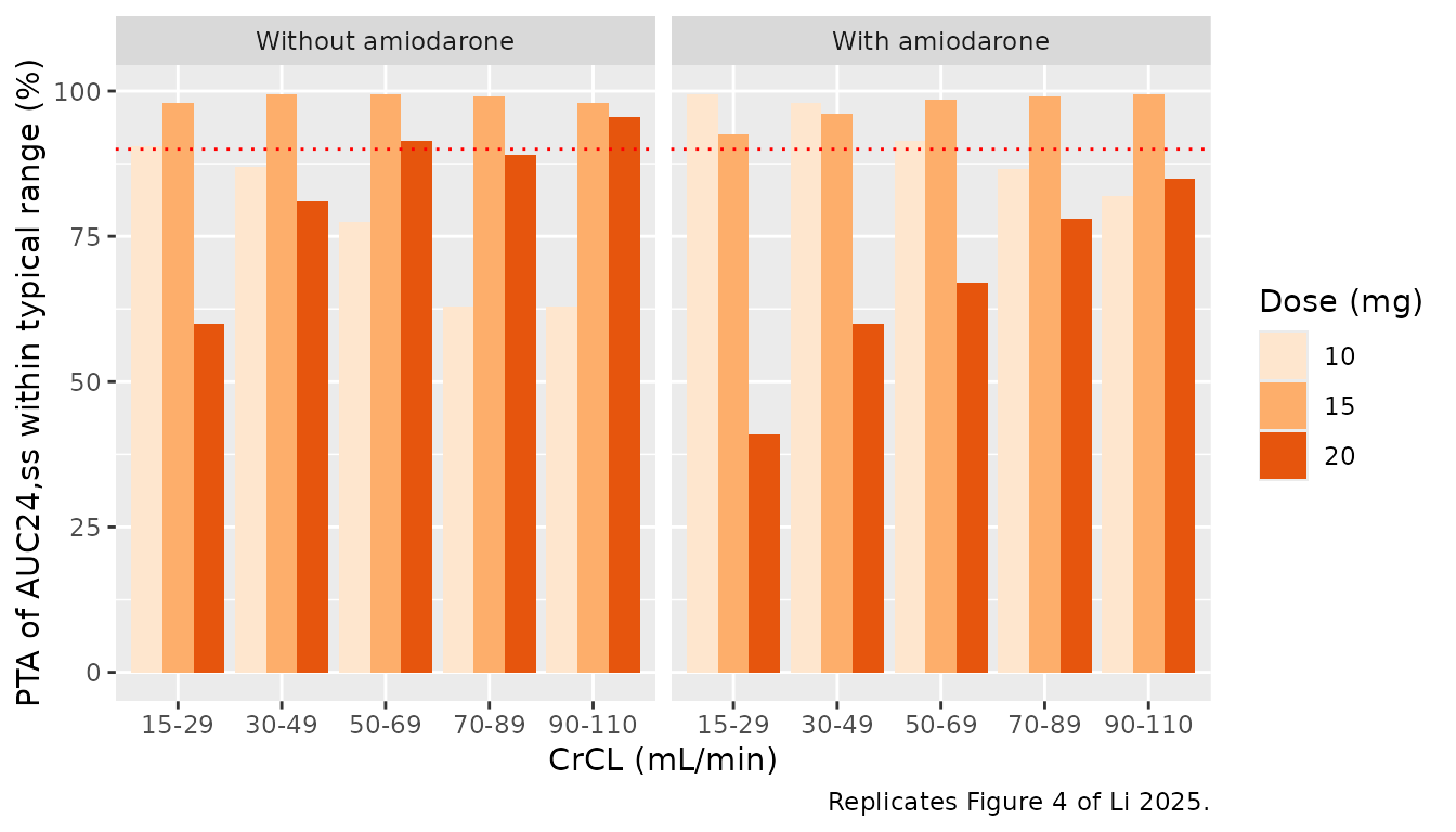
Figure 4 bar heights, digitised by the maintainers (read to roughly +/- 2 percentage points):
fig4_pub <- tibble::tribble(
  ~dose, ~amio,                ~band,    ~pub_pta,
  10,    "Without amiodarone", "15-29",  97,
  10,    "Without amiodarone", "30-49",  91,
  10,    "Without amiodarone", "50-69",  76,
  10,    "Without amiodarone", "70-89",  67,
  10,    "Without amiodarone", "90-110", 57,
  10,    "With amiodarone",    "15-29", 100,
  10,    "With amiodarone",    "30-49",  98,
  10,    "With amiodarone",    "50-69",  99,
  10,    "With amiodarone",    "70-89",  94,
  10,    "With amiodarone",    "90-110", 94,
  15,    "Without amiodarone", "15-29",  97,
  15,    "Without amiodarone", "30-49", 100,
  15,    "Without amiodarone", "50-69", 100,
  15,    "Without amiodarone", "70-89", 100,
  15,    "Without amiodarone", "90-110", 98,
  15,    "With amiodarone",    "15-29",  77,
  15,    "With amiodarone",    "30-49",  87,
  15,    "With amiodarone",    "50-69",  88,
  15,    "With amiodarone",    "70-89",  98,
  15,    "With amiodarone",    "90-110", 97,
  20,    "Without amiodarone", "15-29",  64,
  20,    "Without amiodarone", "30-49",  88,
  20,    "Without amiodarone", "50-69",  90,
  20,    "Without amiodarone", "70-89",  96,
  20,    "Without amiodarone", "90-110", 96,
  20,    "With amiodarone",    "15-29",  19,
  20,    "With amiodarone",    "30-49",  41,
  20,    "With amiodarone",    "50-69",  63,
  20,    "With amiodarone",    "70-89",  69,
  20,    "With amiodarone",    "90-110", 75
)

f4_chk <- fig4_pub |>
  left_join(f3_sim |> select(dose, amio, band, pta), by = c("dose", "amio", "band")) |>
  mutate(diff_pp = pta - pub_pta)

f4_chk |>
  rename(
    "Dose (mg)" = dose,
    "Amiodarone" = amio,
    "CrCL band (mL/min)" = band,
    "Figure 4 PTA (%)" = pub_pta,
    "Simulated PTA (%)" = pta,
    "Difference (pp)" = diff_pp
  ) |>
knitr::kable(digits = 1, caption = "Probability of target attainment, simulated versus Figure 4 of Li 2025.")| Dose (mg) | Amiodarone | CrCL band (mL/min) | Figure 4 PTA (%) | Simulated PTA (%) | Difference (pp) |
|---|---|---|---|---|---|
| 10 | Without amiodarone | 15-29 | 97 | 90.5 | -6.5 |
| 10 | Without amiodarone | 30-49 | 91 | 87.0 | -4.0 |
| 10 | Without amiodarone | 50-69 | 76 | 77.5 | 1.5 |
| 10 | Without amiodarone | 70-89 | 67 | 63.0 | -4.0 |
| 10 | Without amiodarone | 90-110 | 57 | 63.0 | 6.0 |
| 10 | With amiodarone | 15-29 | 100 | 99.5 | -0.5 |
| 10 | With amiodarone | 30-49 | 98 | 98.0 | 0.0 |
| 10 | With amiodarone | 50-69 | 99 | 91.5 | -7.5 |
| 10 | With amiodarone | 70-89 | 94 | 86.5 | -7.5 |
| 10 | With amiodarone | 90-110 | 94 | 82.0 | -12.0 |
| 15 | Without amiodarone | 15-29 | 97 | 98.0 | 1.0 |
| 15 | Without amiodarone | 30-49 | 100 | 99.5 | -0.5 |
| 15 | Without amiodarone | 50-69 | 100 | 99.5 | -0.5 |
| 15 | Without amiodarone | 70-89 | 100 | 99.0 | -1.0 |
| 15 | Without amiodarone | 90-110 | 98 | 98.0 | 0.0 |
| 15 | With amiodarone | 15-29 | 77 | 92.5 | 15.5 |
| 15 | With amiodarone | 30-49 | 87 | 96.0 | 9.0 |
| 15 | With amiodarone | 50-69 | 88 | 98.5 | 10.5 |
| 15 | With amiodarone | 70-89 | 98 | 99.0 | 1.0 |
| 15 | With amiodarone | 90-110 | 97 | 99.5 | 2.5 |
| 20 | Without amiodarone | 15-29 | 64 | 60.0 | -4.0 |
| 20 | Without amiodarone | 30-49 | 88 | 81.0 | -7.0 |
| 20 | Without amiodarone | 50-69 | 90 | 91.5 | 1.5 |
| 20 | Without amiodarone | 70-89 | 96 | 89.0 | -7.0 |
| 20 | Without amiodarone | 90-110 | 96 | 95.5 | -0.5 |
| 20 | With amiodarone | 15-29 | 19 | 41.0 | 22.0 |
| 20 | With amiodarone | 30-49 | 41 | 60.0 | 19.0 |
| 20 | With amiodarone | 50-69 | 63 | 67.0 | 4.0 |
| 20 | With amiodarone | 70-89 | 69 | 78.0 | 9.0 |
| 20 | With amiodarone | 90-110 | 75 | 85.0 | 10.0 |
stopifnot(
  !anyNA(f4_chk$pta),
  abs(median(f4_chk$diff_pp)) < 8,
  quantile(abs(f4_chk$diff_pp), 0.75) < 20
)
The Figure 3 medians are reproduced within a few percent in every cell, and the Figure 3 spread (Q3/Q1 near 1.3) is reproduced too. Figure 4 agrees less closely: 25 of the 30 cells lie within 10 percentage points of the published bar. The broad dosing picture holds: 15 mg once daily keeps PTA at or above 98% in every band without amiodarone, and 20 mg once daily with amiodarone falls well short in renal impairment.
Two things limit the cell-by-cell match, and neither points to a transcription error in the model. First, PTA is the tail mass of a distribution beyond a fixed cut-off, so a few-percent shift of a median that sits near 1860 or 5434 ngh/mL moves PTA by many percentage points. Second, some Figure 4 bars cannot be reconciled with the paper’s own Figure 3. For 20 mg with amiodarone at CrCL 15-29 mL/min, Figure 3c shows a median of about 5650 ngh/mL, above the 5434 upper bound, and a first quartile of about 4900, below it, with the lower whisker well above 1860. Between 25% and 50% of that cell must therefore be in range, but Figure 4 reports 19%. The simulation, which matches Figure 3, gives 41%. The published PTAs in the with-amiodarone panel are generally lower than the simulated ones at high exposure, so the paper’s PTA calculation appears to have used a wider distribution than its Figure 3 shows. Its dosing conclusions for 10 mg with amiodarone (PTA above 90% at CrCL of 50 mL/min or more) are therefore somewhat more optimistic than this model gives.
Steady-state profiles and PKNCA
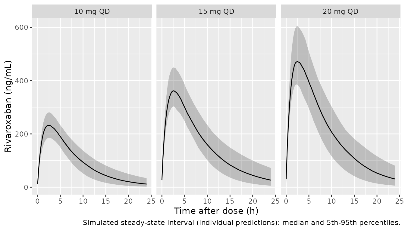
A virtual cohort resembling Table 1 is dosed to steady state with each of the three regimens, and PKNCA is run on the final dosing interval.
set.seed(20251204)
n_per_arm <- 150L
tau <- 24
n_doses <- 10L
t_last <- (n_doses - 1L) * tau

make_arm <- function(n, dose, offset) {
  tibble(
    id = offset + seq_len(n),
    treatment = paste(dose, "mg QD"),
    dose_mg = dose,
    # Table 1: CrCL median 48.6 mL/min, range 14.3-91.7.
    CRCL = pmin(91.7, pmax(14.3, stats::rlnorm(n, log(48.6), 0.4))),
    CONMED_AMIO = stats::rbinom(n, 1L, 0.484)   # 48.4%, Table 1
  )
}

cov_ss <- bind_rows(
  make_arm(n_per_arm, 10, 0L),
  make_arm(n_per_arm, 15, n_per_arm),
  make_arm(n_per_arm, 20, 2L * n_per_arm)
)

obs_times <- t_last + sort(unique(c(seq(0, 6, by = 0.25), seq(6, tau, by = 1))))

ev_ss <- bind_rows(
  cov_ss |>
    tidyr::expand_grid(k = seq_len(n_doses)) |>
    transmute(id, treatment, time = (k - 1L) * tau, evid = 1L, amt = dose_mg,
              cmt = "depot", CRCL, CONMED_AMIO),
  cov_ss |>
    tidyr::expand_grid(time = obs_times) |>
    transmute(id, treatment, time, evid = 0L, amt = NA_real_,
              cmt = "central", CRCL, CONMED_AMIO)
) |>
  arrange(id, time, desc(evid))

rxode2::rxSetSeed(20251204)
sim_ss <- rxode2::rxSolve(mod, events = ev_ss, keep = "treatment") |>
  as.data.frame()

ipar <- sim_ss |> distinct(id, treatment, cl, vc)
stopifnot(nrow(ipar) == 3L * n_per_arm)
sim_ss |>
  mutate(tad = time - t_last) |>
  group_by(treatment, tad) |>
  summarise(
    Q05 = quantile(Cc, 0.05), Q50 = median(Cc), Q95 = quantile(Cc, 0.95),
    .groups = "drop"
  ) |>
  ggplot(aes(tad, Q50)) +
  geom_ribbon(aes(ymin = Q05, ymax = Q95), alpha = 0.25) +
  geom_line() +
  facet_wrap(~treatment) +
  labs(
    x = "Time after dose (h)",
    y = "Rivaroxaban (ng/mL)",
    caption = "Simulated steady-state interval (individual predictions): median and 5th-95th percentiles."
  )
ss_conc <- sim_ss |>
  filter(!is.na(Cc)) |>
  select(id, time, Cc, treatment)

ss_dose <- ev_ss |>
  filter(evid == 1L, time == t_last) |>
  select(id, time, amt, treatment)

conc_obj <- PKNCA::PKNCAconc(ss_conc, Cc ~ time | treatment + id)
dose_obj <- PKNCA::PKNCAdose(ss_dose, amt ~ time | treatment + id)

intervals <- data.frame(
  start = t_last, end = t_last + tau,
  cmax = TRUE, tmax = TRUE, cmin = TRUE, auclast = TRUE
)

nca_res <- PKNCA::pk.nca(PKNCA::PKNCAdata(conc_obj, dose_obj, intervals = intervals))

nca_wide <- as.data.frame(nca_res) |>
  select(id, treatment, PPTESTCD, PPORRES) |>
  tidyr::pivot_wider(names_from = PPTESTCD, values_from = PPORRES)

summary(nca_res)
#>  start end treatment   N     auclast       cmax        cmin              tmax
#>    216 240  10 mg QD 150 2220 [21.0] 233 [13.3]  10.9 [107] 2.50 [2.00, 3.00]
#>    216 240  15 mg QD 150 3710 [20.3] 365 [12.9] 23.6 [91.2] 2.50 [2.00, 3.00]
#>    216 240  20 mg QD 150 4730 [23.0] 481 [13.8]  26.6 [104] 2.50 [2.00, 3.00]
#>
#> Caption: auclast, cmax, cmin: geometric mean and geometric coefficient of variation; tmax: median and range; N: number of subjects
At steady state the interval AUC equals Dose / (CL/F),
which is how Li 2025 derived the individual AUC24,ss used
in Figures 3-6. Both sides of this check use the same drawn clearances,
so the difference is numerical (trapezoidal error around the absorption
peak) and a tight bound applies.
auc_chk <- nca_wide |>
  left_join(ipar, by = c("id", "treatment")) |>
  left_join(cov_ss |> select(id, dose_mg), by = "id") |>
  mutate(
    auc_closed = 1000 * dose_mg / cl,
    pct = 100 * (auclast / auc_closed - 1)
  )

knitr::kable(
  auc_chk |>
    summarise(
      "Median abs % diff" = median(abs(pct)),
      "Max abs % diff" = max(abs(pct))
    ),
  digits = 3,
  caption = "PKNCA AUC0-24,ss against Dose / (CL/F) for the same simulated subjects."
)| Median abs % diff | Max abs % diff |
|---|---|
| 0.071 | 0.163 |
Comparison against published exposure
Li 2025 does not report NCA parameters. Its Figure 5a gives the
arithmetic mean post-hoc AUC24,ss per dose group in the 80
patients of the exposure-response analysis (bar heights digitised by the
maintainers: 10 mg about 2380, 15 mg about 3230, 20 mg about 3820
ng*h/mL; the 20 mg group has only 3 patients).
published <- tibble::tribble(
  ~treatment, ~auclast,
  "10 mg QD",  2380,
  "15 mg QD",  3230,
  "20 mg QD",  3820
)

nlmixr2lib::ncaComparisonTable(
  simulated = nca_res,
  reference = published,
  by = "treatment",
  units = c(auclast = "ng*h/mL", cmax = "ng/mL", cmin = "ng/mL", tmax = "h"),
  tolerance_pct = 20
) |>
  knitr::kable(caption = paste(
    "Simulated steady-state NCA (median) versus the Figure 5a mean post-hoc",
    "AUC24,ss of Li 2025. Cmax, Cmin and Tmax have no published counterpart.",
    "* differs from reference by more than 20%."
))| NCA parameter | treatment | Reference | Simulated | % diff |
|---|---|---|---|---|
| AUClast (ng*h/mL) | 10 mg QD | 2380 | 2200 | -7.4% |
| AUClast (ng*h/mL) | 15 mg QD | 3230 | 3640 | +12.7% |
| AUClast (ng*h/mL) | 20 mg QD | 3820 | 4770 | +24.9%* |
The 10 and 15 mg groups agree to within about 15%, and the 20 mg
group lies higher. This comparison is confounded by design: the virtual
cohort assigns every regimen the whole Table 1 covariate distribution,
whereas in the study the clinician chose each patient’s dose. Patients
given the higher doses presumably had better renal function than the
cohort as a whole, which lowers their AUC, and the 20 mg group has only
three patients. The mean-versus-median difference is negligible here
(about 2% at omega^2 = 0.036). The same confounding
explains why Figure 5b reports with/without-amiodarone AUC ratios of
1.17 (10 mg) and 1.25 (15 mg) while the model’s amiodarone effect alone
is exp(0.124) = 1.13.
Exposure-response findings
The exposure-response part of Li 2025 is descriptive and contributes
no model parameters: patients with thromboembolic events had lower
AUC24,ss (2311 vs 2818 ngh/mL), a ROC analysis gave
2840 ngh/mL as a cut-off (AUC 0.70, 95% CI 0.55-0.84), and patients
with clinically relevant non-major bleeding had higher
AUC24,ss (3378 vs 2531 ng*h/mL) (Results “Exposure-Response
Results”). These can be applied to the simulated AUC24,ss
above but are not part of the model.
Assumptions and deviations
-
IIV magnitude. Table 2 labels the IIV rows “omega2
CL (%)” and “omega2 V (%)” with values 3.6 and 3.3. They are encoded as
variances 0.036 and 0.033 (CV about 19% and 18%). The reading is
confirmed by the paper’s own simulation: within one CrCL band, Figure 3
boxes have Q3/Q1 near 1.3, which matches
omega^2 = 0.036; reading the values as 3.6% CV would give about 1.05. - CrCL reference value. The Table 2 footnote equation centres CrCL at 47.4 mL/min, while Table 1 reports a cohort median of 48.6 mL/min. The value printed in the equation is used. The difference changes the typical CL/F by less than 0.5%.
- CrCL units. Cockcroft-Gault creatinine clearance in mL/min, not normalised to body surface area, as in the sibling rivaroxaban models in this package.
- Fixed ka. Li 2025 fixed ka at 0.821 1/h from its references 28 and 29.
-
Residual error. Phoenix
stdev0is taken as an additive SD in ng/mL, the concentration unit used throughout the paper. - CrCL within simulation bands. Li 2025 does not describe the CrCL distribution inside each band of its Figure 3/4 simulation; a uniform distribution across the band is used here.
- Steady-state cohort. CrCL is drawn log-normal (median 48.6 mL/min, truncated to the observed range 14.3-91.7) and amiodarone use with probability 0.484, matching Table 1; the paper gives no further distributional detail.