Dexamethasone and betamethasone IM and oral (Krzyzanski 2021) • nlmixr2lib

Model and source

Krzyzanski et al. (2021) fitted the dexamethasone (DEX) and betamethasone (BET) data independently, each with its own two-compartment model, so the paper contributes two model files that share this vignette:

Krzyzanski_2021_dexamethasone: Two-compartment population PK model for dexamethasone after single 6 mg doses of dexamethasone phosphate given intramuscularly or orally to healthy nonpregnant Indian women, with separate first-order absorption from an IM and an oral depot. Clearances and volumes are apparent (divided by the IM bioavailability FIM); oral bioavailability is relative to IM (Fr = FPO / FIM). No covariates.
Krzyzanski_2021_betamethasone: Two-compartment population PK model for betamethasone after single 6 mg doses of betamethasone phosphate given intramuscularly or orally, or of a 1:1 betamethasone phosphate/acetate IM suspension (Celestone), to healthy nonpregnant Indian women. Three parallel first-order absorption depots: IM phosphate, oral phosphate, and a slow IM acetate depot (flip-flop terminal phase). Clearances and volumes are apparent (divided by the IM bioavailability FIM); oral and acetate bioavailabilities are relative to IM phosphate. No covariates.
Citation: Krzyzanski W, Milad MA, Jobe AH, Peppard T, Bies RR, Jusko WJ. Population pharmacokinetic modeling of intramuscular and oral dexamethasone and betamethasone in Indian women. J Pharmacokinet Pharmacodyn. 2021;48(2):261-272. doi:10.1007/s10928-020-09730-z
Article (open access): https://doi.org/10.1007/s10928-020-09730-z
Supplement (NONMEM control stream for BET; Tables S1-S2): Electronic Supplementary Material 1 and 2 of the article.

Population

Forty-eight healthy, nonpregnant Indian women (ages 22-39 years, body weight 47.0-68.7 kg, mean 56.8 kg, BMI 20.6-25.0 kg/m^2) took part in an open-label, randomized, two-period partial crossover study (NCT03668860; Krzyzanski 2021 Tables 1-2). Each woman received two of five single-dose treatments, each delivering 6 mg of the free-alcohol steroid:

Treatment	Route	Formulation	n
A (DEX-P IM)	IM	dexamethasone phosphate solution	12
B (BET-P IM)	IM	betamethasone phosphate solution	12
C (BET-PA IM)	IM	3 mg betamethasone phosphate + 3 mg betamethasone acetate suspension (Celestone)	24
D (DEX-P PO)	PO	0.5 mg dexamethasone phosphate tablets	24
E (BET-P PO)	PO	0.5 mg betamethasone phosphate tablets	24

Plasma was sampled to 96 h after each dose. The DEX model was fitted to 578 concentrations (103 below the 0.1 ng/mL LLOQ) from the 36 women who received DEX; the BET model to 949 concentrations (19 below LLOQ) from all 48 women. The homogeneous population precluded a covariate analysis, so neither model carries covariates. The same information is available programmatically via readModelDb("Krzyzanski_2021_dexamethasone")()$population.

Source trace

Model equations are Krzyzanski 2021 Eqs 1-7 (structure), Eq 10 (log-normal IIV) and Eq 11 (additive residual error on log concentrations, i.e. lnorm). The supplement’s BET NONMEM control stream confirms the structure: five compartments (IM, plasma, peripheral, PO, IM acetate), F4 = FR, F5 = FRA, the IM phosphate depot as the bioavailability reference, and Y = LOG(A(2)/V) + EPS(1).

Parameter	DEX	BET	Source location
`lcl` CL/FIM (L/h)	9.29	5.95	Tables 3 / 4; BET supplement `$THETA 1`
`lvc` Vp/FIM (L)	51.3	67.5	Tables 3 / 4; `$THETA 2`
`lq` CLD/FIM (L/h)	0.538	0.173	Tables 3 / 4; `$THETA 8`
`lvp` VT/FIM (L)	5.06	4.94	Tables 3 / 4; `$THETA 9`
`lka_im` kaIM (1/h)	0.460	0.971	Tables 3 / 4; `$THETA 3`
`lka_oral` kaPO (1/h)	0.936	1.21	Tables 3 / 4; `$THETA 5`
`lka_im_acetate` kaIMa (1/h)	–	0.00638	Table 4; `$THETA 4`
`lfdepot_oral` Fr = FPO/FIM	1.04	0.935	Tables 3 / 4, Eq 7; `$THETA 6`
`lfdepot_im_acetate` Fra = FIMa/FIM	–	0.819	Table 4, Eq 7; `$THETA 7`
`etalcl` omega^2	0.0265	0.0210	Tables 3 / 4
`etalvc` omega^2	0 (fixed; omitted)	0.0188	Tables 3 / 4
cov(`etalcl`, `etalvc`)	–	0.0155	Table 4; `$OMEGA BLOCK(2)`
`etalka_im` omega^2	0.0633	0.0441	Tables 3 / 4
`etalka_oral` omega^2	0.395	0.241	Tables 3 / 4
`etalka_im_acetate` omega^2	–	0.147	Table 4
`etalfdepot_oral` omega^2	–	0.0182	Table 4
`etalfdepot_im_acetate` omega^2	–	0.00773	Table 4
`expSd` = sqrt(sigma^2)	sqrt(0.0455)	sqrt(0.0211)	Tables 3 / 4; `$SIGMA`

The steady-state volumes quoted in the abstract are reproduced from the table values: Vss/FIM = 51.3 + 5.06 = 56.4 L (DEX) and 67.5 + 4.94 = 72.4 L (BET).

dex_ini <- rxode2::rxode(readModelDb("Krzyzanski_2021_dexamethasone"))$iniDf
#> ℹ parameter labels from comments will be replaced by 'label()'
bet_ini <- rxode2::rxode(readModelDb("Krzyzanski_2021_betamethasone"))$iniDf
#> ℹ parameter labels from comments will be replaced by 'label()'
theta <- function(ini, nm) exp(ini$est[ini$name == nm])
vss <- c(
  DEX = theta(dex_ini, "lvc") + theta(dex_ini, "lvp"),
  BET = theta(bet_ini, "lvc") + theta(bet_ini, "lvp")
)
vss
#>   DEX   BET 
#> 56.36 72.44
# Abstract: Vss/FIM = 56.4 L (DEX) and 72.4 L (BET).
stopifnot(abs(vss - c(56.4, 72.4)) < 0.05)

Dosing the models

Both models use numbered parallel absorption depots. Doses are in mg of the free-alcohol steroid and Cc is in ng/mL.

Compartment	Route / formulation	Bioavailability
`depot1`	IM phosphate (DEX-P or BET-P)	1 (reference, FIM)
`depot2`	oral phosphate tablets	`Fr`
`depot3`	IM acetate (BET model only)	`Fra`

A Celestone (BET-PA) injection is split between two depots: half of the dose as phosphate into depot1 and half as acetate into depot3.

Virtual cohort and simulation of the five treatments

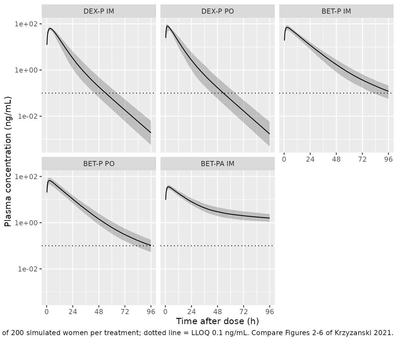
The observed data are not public. Each treatment is simulated in 200 virtual women over the 96 h sampling window. No covariates are needed.

rxode2::rxSetSeed(20210103)
n_arm <- 200L
obs_times <- sort(unique(c(seq(0, 6, by = 0.25), 7:96)))

# One cohort as a self-contained event table. `id_offset` keeps subject IDs
# disjoint across arms so rxSolve cannot merge subjects.
make_arm <- function(n, treatment, cmts, amts, dose_times = 0, id_offset = 0L) {
  ids <- id_offset + seq_len(n)
  doses <- tidyr::expand_grid(
    id = ids,
    time = dose_times,
    dose_row = seq_along(cmts)
  ) |>
    mutate(
      evid = 1L,
      cmt = cmts[dose_row],
      amt = amts[dose_row]
    ) |>
    select(-dose_row)
  obs <- tidyr::expand_grid(id = ids, time = obs_times) |>
    mutate(evid = 0L, cmt = "central", amt = 0)
  bind_rows(doses, obs) |>
    mutate(treatment = treatment) |>
    arrange(id, time, desc(evid))
}

events_dex <- bind_rows(
  make_arm(n_arm, "DEX-P IM", "depot1", 6, id_offset = 0L),
  make_arm(n_arm, "DEX-P PO", "depot2", 6, id_offset = n_arm)
)
events_bet <- bind_rows(
  make_arm(n_arm, "BET-P IM", "depot1", 6, id_offset = 0L),
  make_arm(n_arm, "BET-P PO", "depot2", 6, id_offset = n_arm),
  make_arm(n_arm, "BET-PA IM", c("depot1", "depot3"), c(3, 3), id_offset = 2L * n_arm)
)
stopifnot(
  !anyDuplicated(unique(events_dex[, c("id", "time", "evid", "cmt")])),
  !anyDuplicated(unique(events_bet[, c("id", "time", "evid", "cmt")]))
)

mod_dex <- readModelDb("Krzyzanski_2021_dexamethasone")
mod_bet <- readModelDb("Krzyzanski_2021_betamethasone")

sim_dex <- rxode2::rxSolve(mod_dex, events = events_dex, keep = "treatment") |>
  as.data.frame()
#> ℹ parameter labels from comments will be replaced by 'label()'
sim_bet <- rxode2::rxSolve(mod_bet, events = events_bet, keep = "treatment") |>
  as.data.frame()
#> ℹ parameter labels from comments will be replaced by 'label()'

sim_all <- bind_rows(
  sim_dex |> mutate(id = id, drug = "DEX"),
  sim_bet |> mutate(id = id + 10000L, drug = "BET")
) |>
  mutate(treatment = factor(
    treatment,
    levels = c("DEX-P IM", "DEX-P PO", "BET-P IM", "BET-P PO", "BET-PA IM")
  ))

Replicate Figures 2-6

# Replicates the model-predicted bands of the VPCs in Figures 3-6 of
# Krzyzanski 2021 (median and 5th-95th percentiles by treatment); Figure 2 is
# the matching observed-data spaghetti plot.
sim_all |>
  filter(time > 0) |>
  group_by(treatment, time) |>
  summarise(
    Q05 = quantile(Cc, 0.05),
    Q50 = quantile(Cc, 0.50),
    Q95 = quantile(Cc, 0.95),
    .groups = "drop"
  ) |>
  ggplot(aes(time, Q50)) +
  geom_ribbon(aes(ymin = Q05, ymax = Q95), alpha = 0.25) +
  geom_line() +
  geom_hline(yintercept = 0.1, linetype = "dotted") +
  facet_wrap(~treatment) +
  scale_y_log10() +
  scale_x_continuous(breaks = seq(0, 96, by = 24)) +
  labs(
    x = "Time after dose (h)", y = "Plasma concentration (ng/mL)",
    caption = paste(
      "Median and 5th-95th percentiles of 200 simulated women per treatment;",
      "dotted line = LLOQ 0.1 ng/mL. Compare Figures 2-6 of Krzyzanski 2021."
    )
  )

PKNCA validation against Supplementary Table S1

Supplementary Table S1 lists the mean (SD) over individual model predictions of Cmax, tmax and terminal half-life for each treatment, where the paper took the half-life from the 95 and 96 h points only. PKNCA computes Cmax, tmax and the half-life with its automatic terminal-phase selection. The paper’s two-point half-life is computed separately below.

sim_nca <- sim_all |>
  filter(!is.na(Cc)) |>
  select(id, time, Cc, treatment)
# Guarantee a time-zero row per subject (pre-dose Cc = 0 for extravascular).
sim_nca <- bind_rows(
  sim_nca,
  sim_nca |> distinct(id, treatment) |> mutate(time = 0, Cc = 0)
) |>
  distinct(id, treatment, time, .keep_all = TRUE) |>
  arrange(treatment, id, time)

dose_df <- bind_rows(
  events_dex |> mutate(id = id),
  events_bet |> mutate(id = id + 10000L)
) |>
  filter(evid == 1) |>
  group_by(id, time, treatment) |>
  summarise(amt = sum(amt), .groups = "drop")

conc_obj <- PKNCA::PKNCAconc(sim_nca, Cc ~ time | treatment + id,
                             concu = "ng/mL", timeu = "h")
dose_obj <- PKNCA::PKNCAdose(dose_df, amt ~ time | treatment + id,
                             doseu = "mg")
intervals <- data.frame(
  start = 0, end = 96,
  cmax = TRUE, tmax = TRUE, half.life = TRUE
)
nca_res <- PKNCA::pk.nca(PKNCA::PKNCAdata(conc_obj, dose_obj, intervals = intervals))

# Table S1 reports means of individual values, so the simulated side is
# aggregated with the mean as well (ncaComparisonTable() defaults to median).
sim_mean <- as.data.frame(nca_res$result) |>
  filter(PPTESTCD %in% c("cmax", "tmax", "half.life")) |>
  group_by(treatment, PPTESTCD) |>
  summarise(PPORRES = mean(PPORRES, na.rm = TRUE), .groups = "drop")

published_s1 <- tibble::tribble(
  ~treatment,  ~cmax, ~tmax, ~half.life,
  "DEX-P IM",   62.5,  3.3,   7.5,
  "DEX-P PO",   78.9,  2.2,   7.6,
  "BET-P IM",   66.9,  2.8,  14.9,
  "BET-P PO",   65.9,  2.6,  18.7,
  "BET-PA IM",  35.8,  2.9,  77.6
)

cmp <- nlmixr2lib::ncaComparisonTable(
  simulated = sim_mean,
  reference = published_s1,
  by = "treatment",
  units = c(cmax = "ng/mL", tmax = "h", half.life = "h"),
  tolerance_pct = 20
)
knitr::kable(
  cmp,
  caption = "Simulated (mean of 200 per treatment) vs. Krzyzanski 2021 Table S1. * differs by >20%."
)

Simulated (mean of 200 per treatment) vs. Krzyzanski 2021 Table S1. * differs by >20%.
NCA parameter	treatment	Reference	Simulated	% diff
Cmax (ng/mL)	DEX-P IM	62.5	63	+0.9%
Cmax (ng/mL)	DEX-P PO	78.9	79.5	+0.8%
Cmax (ng/mL)	BET-P IM	66.9	70.9	+5.9%
Cmax (ng/mL)	BET-P PO	65.9	68.1	+3.4%
Cmax (ng/mL)	BET-PA IM	35.8	35.8	-0.1%
Tmax (h)	DEX-P IM	3.3	3.29	-0.3%
Tmax (h)	DEX-P PO	2.2	2.33	+6.0%
Tmax (h)	BET-P IM	2.8	2.72	-2.8%
Tmax (h)	BET-P PO	2.6	2.52	-3.1%
Tmax (h)	BET-PA IM	2.9	2.83	-2.5%
t½ (h)	DEX-P IM	7.5	7.26	-3.2%
t½ (h)	DEX-P PO	7.6	7.24	-4.7%
t½ (h)	BET-P IM	14.9	16.6	+11.6%
t½ (h)	BET-P PO	18.7	16.8	-10.3%
t½ (h)	BET-PA IM	77.6	88.4	+13.9%

chk <- sim_mean |>
  filter(PPTESTCD == "cmax") |>
  inner_join(published_s1, by = "treatment") |>
  mutate(pct_diff = 100 * (PPORRES - cmax) / cmax)
chk
#> # A tibble: 5 × 7
#>   treatment PPTESTCD PPORRES  cmax  tmax half.life pct_diff
#>   <chr>     <chr>      <dbl> <dbl> <dbl>     <dbl>    <dbl>
#> 1 BET-P IM  cmax        70.9  66.9   2.8      14.9   5.93  
#> 2 BET-P PO  cmax        68.1  65.9   2.6      18.7   3.38  
#> 3 BET-PA IM cmax        35.8  35.8   2.9      77.6  -0.0677
#> 4 DEX-P IM  cmax        63.0  62.5   3.3       7.5   0.859 
#> 5 DEX-P PO  cmax        79.5  78.9   2.2       7.6   0.763
# Mean Cmax over 200 subjects is a centre statistic. A mis-transcribed
# clearance, volume, ka or bioavailability moves it by tens of percent.
stopifnot(all(abs(chk$pct_diff) < 12))

The Table S1 half-life used only the 95 and 96 h points. Reproducing that definition:

hl_95_96 <- sim_all |>
  filter(time %in% c(95, 96)) |>
  select(treatment, id, time, Cc) |>
  tidyr::pivot_wider(names_from = time, values_from = Cc, names_prefix = "C") |>
  mutate(thalf = log(2) / log(C95 / C96)) |>
  group_by(treatment) |>
  summarise(mean_thalf = mean(thalf), sd_thalf = sd(thalf), .groups = "drop") |>
  inner_join(published_s1 |> select(treatment, published = half.life), by = "treatment")
hl_95_96 |>
  dplyr::rename(
    "Treatment" = treatment,
    "Simulated mean t1/2 (h)" = mean_thalf,
    "Simulated SD (h)" = sd_thalf,
    "Table S1 mean t1/2 (h)" = published
  ) |>
  knitr::kable(digits = 1)

Treatment	Simulated mean t1/2 (h)	Simulated SD (h)	Table S1 mean t1/2 (h)
DEX-P IM	7.4	0.3	7.5
DEX-P PO	7.3	0.2	7.6
BET-P IM	17.1	1.0	14.9
BET-P PO	17.2	0.9	18.7
BET-PA IM	90.6	24.7	77.6

For DEX-P IM and PO, BET-P IM and BET-P PO the two-point half-life matches the paper to within about 15%. The BET-PA IM value is longer than Table S1 reports (77.6 h). With the typical parameters, the 95-96 h slope still mixes the 17 h disposition phase and the 109 h acetate absorption phase, and the simulated mean lies between them. Table S1 averages the post-hoc estimates of the 24 women who received BET-PA, whereas this is a fresh simulation from the population estimates. See Assumptions and deviations.

Mean residence time (Eq 9)

The paper defines MRT = (Vss/FIM)/(CL/FIM) + 1/ka, with the effective ka for BET-PA combining the two IM depots weighted by their bioavailabilities.

mrt <- sim_all |>
  filter(time == 0) |>
  distinct(id, .keep_all = TRUE) |>
  mutate(
    ka_eff = case_when(
      treatment %in% c("DEX-P IM", "BET-P IM") ~ ka_im,
      treatment %in% c("DEX-P PO", "BET-P PO") ~ ka_oral,
      treatment == "BET-PA IM" ~ (1 + fra) / (1 / ka_im + fra / ka_im_acetate)
    ),
    mrt = (vc + vp) / cl + 1 / ka_eff
  ) |>
  group_by(treatment) |>
  summarise(mean_mrt = mean(mrt), sd_mrt = sd(mrt), .groups = "drop") |>
  mutate(published = c(7.81, 6.91, 12.1, 12.5, 96.5)[match(
    treatment, c("DEX-P IM", "DEX-P PO", "BET-P IM", "BET-P PO", "BET-PA IM")
  )])
mrt |>
  dplyr::rename(
    "Treatment" = treatment,
    "Simulated mean MRT (h)" = mean_mrt,
    "Simulated SD (h)" = sd_mrt,
    "Table S1 mean MRT (h)" = published
  ) |>
  knitr::kable(digits = 2)

Treatment	Simulated mean MRT (h)	Simulated SD (h)	Table S1 mean MRT (h)
DEX-P IM	8.38	1.15	7.81
DEX-P PO	7.51	1.42	6.91
BET-P IM	13.36	1.19	12.10
BET-P PO	12.98	1.09	12.50
BET-PA IM	86.98	30.19	96.50

The simulated mean MRTs are within about 10% of Table S1.

Mass balance

With the random effects removed, AUC(0-inf) x CL/FIM must equal the bioavailable dose. This check does not depend on random draws.

typ_dex <- rxode2::zeroRe(mod_dex)
#> ℹ parameter labels from comments will be replaced by 'label()'
typ_bet <- rxode2::zeroRe(mod_bet)
#> ℹ parameter labels from comments will be replaced by 'label()'
long_grid <- c(seq(0, 24, by = 0.1), seq(25, 4000, by = 1))
mb_events <- function(cmts, amts) {
  bind_rows(
    tibble(id = 1L, time = 0, evid = 1L, cmt = cmts, amt = amts),
    tibble(id = 1L, time = long_grid, evid = 0L, cmt = "central", amt = 0)
  ) |>
    arrange(time, desc(evid))
}
trap <- function(s) sum(diff(s$time) * (head(s$Cc, -1) + tail(s$Cc, -1)) / 2)
mb <- tibble::tribble(
  ~case, ~model, ~cmts, ~amts, ~expected,
  "DEX-P IM", "dex", "depot1", 6, 6 / 9.29,
  "DEX-P PO", "dex", "depot2", 6, 6 * 1.04 / 9.29,
  "BET-P IM", "bet", "depot1", 6, 6 / 5.95,
  "BET-P PO", "bet", "depot2", 6, 6 * 0.935 / 5.95,
  "BET-PA IM", "bet", c("depot1", "depot3"), c(3, 3), (3 + 3 * 0.819) / 5.95
)
mb$simulated <- vapply(seq_len(nrow(mb)), function(i) {
  m <- if (mb$model[i] == "dex") typ_dex else typ_bet
  s <- as.data.frame(rxode2::rxSolve(m, mb_events(mb$cmts[[i]], mb$amts[[i]])))
  # ng*h/mL = ug*h/L; convert to mg*h/L to compare with dose (mg) / CL (L/h)
  trap(s) / 1000
}, numeric(1))
#> ℹ omega/sigma items treated as zero: 'etalcl', 'etalka_im', 'etalka_oral'
#> ℹ omega/sigma items treated as zero: 'etalcl', 'etalka_im', 'etalka_oral'
#> ℹ omega/sigma items treated as zero: 'etalcl', 'etalvc', 'etalka_im', 'etalka_im_acetate', 'etalka_oral', 'etalfdepot_oral', 'etalfdepot_im_acetate'
#> ℹ omega/sigma items treated as zero: 'etalcl', 'etalvc', 'etalka_im', 'etalka_im_acetate', 'etalka_oral', 'etalfdepot_oral', 'etalfdepot_im_acetate'
#> ℹ omega/sigma items treated as zero: 'etalcl', 'etalvc', 'etalka_im', 'etalka_im_acetate', 'etalka_oral', 'etalfdepot_oral', 'etalfdepot_im_acetate'
mb$pct_diff <- 100 * (mb$simulated - mb$expected) / mb$expected
mb |>
  select(case, expected, simulated, pct_diff) |>
  dplyr::rename(
    "Treatment" = case,
    "F x Dose / CL (mg*h/L)" = expected,
    "Simulated AUC0-4000 (mg*h/L)" = simulated,
    "% diff" = pct_diff
  ) |>
  knitr::kable(digits = 3)

Treatment	F x Dose / CL (mg*h/L)	Simulated AUC0-4000 (mg*h/L)	% diff
DEX-P IM	0.646	0.646	-0.001
DEX-P PO	0.672	0.672	-0.010
BET-P IM	1.008	1.008	0.001
BET-P PO	0.943	0.943	-0.001
BET-PA IM	0.917	0.917	0.000

# Same drawn parameters on both sides: only numerical error remains.
stopifnot(all(abs(mb$pct_diff) < 0.5))

Antenatal regimens: Figure 8 and Supplementary Table S2

The paper simulated three WHO antenatal corticosteroid regimens in 200 women each: DEX-P 6 mg IM every 12 h x 4, BET-P 12 mg IM every 24 h x 2, and BET-PA (Celestone) 12 mg IM every 24 h x 2. Table S2 reports the median and 5th-95th percentiles of Cmax, Ctrough and AUC0-48 and AUC0-72.

obs_times <- sort(unique(c(seq(0, 72, by = 0.25))))
events_reg_dex <- make_arm(n_arm, "DEX 6 mg IM 4xBID", "depot1", 6,
                           dose_times = c(0, 12, 24, 36), id_offset = 0L)
events_reg_bet <- bind_rows(
  make_arm(n_arm, "BET 12 mg IM 2xQD", "depot1", 12,
           dose_times = c(0, 24), id_offset = 0L),
  make_arm(n_arm, "CEL 12 mg IM 2xQD", c("depot1", "depot3"), c(6, 6),
           dose_times = c(0, 24), id_offset = n_arm)
)
sim_reg <- bind_rows(
  rxode2::rxSolve(mod_dex, events = events_reg_dex, keep = "treatment") |>
    as.data.frame() |> mutate(id = id),
  rxode2::rxSolve(mod_bet, events = events_reg_bet, keep = "treatment") |>
    as.data.frame() |> mutate(id = id + 10000L)
)

# Replicates Figure 8 of Krzyzanski 2021.
sim_reg |>
  group_by(treatment, time) |>
  summarise(
    Q05 = quantile(Cc, 0.05), Q50 = median(Cc), Q95 = quantile(Cc, 0.95),
    .groups = "drop"
  ) |>
  ggplot(aes(time, Q50, colour = treatment, fill = treatment)) +
  geom_ribbon(aes(ymin = Q05, ymax = Q95), alpha = 0.2, colour = NA) +
  geom_line() +
  scale_x_continuous(breaks = seq(0, 72, by = 12)) +
  labs(
    x = "Time (h)", y = "Plasma concentration (ng/mL)", colour = NULL, fill = NULL,
    caption = "Median and 5th-95th percentiles, 200 women per regimen. Replicates Figure 8 of Krzyzanski 2021."
  ) +
  theme(legend.position = "bottom")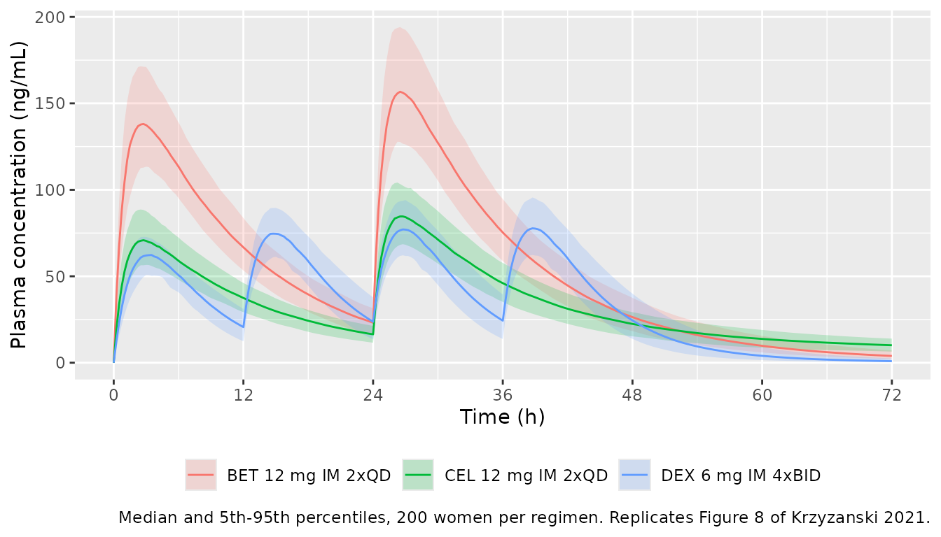

reg_nca <- bind_rows(
  sim_reg |> filter(!is.na(Cc)) |> select(id, time, Cc, treatment),
  sim_reg |> distinct(id, treatment) |> mutate(time = 0, Cc = 0)
) |>
  distinct(id, treatment, time, .keep_all = TRUE) |>
  arrange(treatment, id, time)
reg_dose <- bind_rows(
  events_reg_dex |> mutate(id = id),
  events_reg_bet |> mutate(id = id + 10000L)
) |>
  filter(evid == 1) |>
  group_by(id, time, treatment) |>
  summarise(amt = sum(amt), .groups = "drop")
reg_intervals <- data.frame(
  start = c(0, 0), end = c(48, 72),
  cmax = c(FALSE, TRUE), auclast = c(TRUE, TRUE)
)
reg_res <- PKNCA::pk.nca(PKNCA::PKNCAdata(
  PKNCA::PKNCAconc(reg_nca, Cc ~ time | treatment + id, concu = "ng/mL", timeu = "h"),
  PKNCA::PKNCAdose(reg_dose, amt ~ time | treatment + id, doseu = "mg"),
  intervals = reg_intervals
))

reg_sim_long <- as.data.frame(reg_res$result) |>
  filter(PPTESTCD %in% c("cmax", "auclast")) |>
  mutate(window = paste0("0-", end, " h")) |>
  group_by(treatment, window, PPTESTCD) |>
  summarise(PPORRES = median(PPORRES), .groups = "drop")

published_s2 <- tibble::tribble(
  ~treatment,           ~window,  ~cmax,  ~auclast,
  "DEX 6 mg IM 4xBID",  "0-48 h", NA,     2366,
  "DEX 6 mg IM 4xBID",  "0-72 h", 71.6,   2521,
  "BET 12 mg IM 2xQD",  "0-48 h", NA,     3594,
  "BET 12 mg IM 2xQD",  "0-72 h", 144.2,  3861,
  "CEL 12 mg IM 2xQD",  "0-48 h", NA,     2021,
  "CEL 12 mg IM 2xQD",  "0-72 h", 77.4,   2342
)

cmp_reg <- nlmixr2lib::ncaComparisonTable(
  simulated = reg_sim_long,
  reference = published_s2,
  by = c("treatment", "window"),
  units = c(cmax = "ng/mL", auclast = "ng*h/mL"),
  tolerance_pct = 20
)
knitr::kable(
  cmp_reg,
  caption = "Simulated median vs. Krzyzanski 2021 Table S2 (median of 200). * differs by >20%."
)

Simulated median vs. Krzyzanski 2021 Table S2 (median of 200). * differs by >20%.
NCA parameter	treatment	window	Reference	Simulated	% diff
Cmax (ng/mL)	DEX 6 mg IM 4xBID	0-72 h	71.6	78	+8.9%
Cmax (ng/mL)	BET 12 mg IM 2xQD	0-72 h	144	157	+9.0%
Cmax (ng/mL)	CEL 12 mg IM 2xQD	0-72 h	77.4	84.9	+9.7%
AUClast (ng*h/mL)	DEX 6 mg IM 4xBID	0-48 h	2370	2400	+1.5%
AUClast (ng*h/mL)	DEX 6 mg IM 4xBID	0-72 h	2520	2560	+1.6%
AUClast (ng*h/mL)	BET 12 mg IM 2xQD	0-48 h	3590	3690	+2.8%
AUClast (ng*h/mL)	BET 12 mg IM 2xQD	0-72 h	3860	3980	+3.2%
AUClast (ng*h/mL)	CEL 12 mg IM 2xQD	0-48 h	2020	2120	+5.0%
AUClast (ng*h/mL)	CEL 12 mg IM 2xQD	0-72 h	2340	2460	+5.0%

chk_reg <- reg_sim_long |>
  filter(PPTESTCD == "auclast") |>
  inner_join(published_s2, by = c("treatment", "window")) |>
  mutate(pct_diff = 100 * (PPORRES - auclast) / auclast)
chk_reg
#> # A tibble: 6 × 7
#>   treatment         window PPTESTCD PPORRES  cmax auclast pct_diff
#>   <chr>             <chr>  <chr>      <dbl> <dbl>   <dbl>    <dbl>
#> 1 BET 12 mg IM 2xQD 0-48 h auclast    3694.  NA      3594     2.78
#> 2 BET 12 mg IM 2xQD 0-72 h auclast    3984. 144.     3861     3.18
#> 3 CEL 12 mg IM 2xQD 0-48 h auclast    2123.  NA      2021     5.04
#> 4 CEL 12 mg IM 2xQD 0-72 h auclast    2459.  77.4    2342     5.01
#> 5 DEX 6 mg IM 4xBID 0-48 h auclast    2402.  NA      2366     1.54
#> 6 DEX 6 mg IM 4xBID 0-72 h auclast    2562.  71.6    2521     1.62
# Median AUC over 200 subjects is a centre statistic driven by CL/FIM and the
# relative bioavailabilities; a transcription error moves it by >10%.
stopifnot(all(abs(chk_reg$pct_diff) < 10))

Trough concentrations (Table S2 Ctrough; the paper does not state the time at which the trough was taken):

published_ctrough <- c(
  "BET 12 mg IM 2xQD" = 26.4, "CEL 12 mg IM 2xQD" = 17.1, "DEX 6 mg IM 4xBID" = 33.1
)
sim_reg |>
  filter(time %in% c(12, 24, 36, 48)) |>
  group_by(treatment, time) |>
  summarise(median_Cc = median(Cc), .groups = "drop") |>
  tidyr::pivot_wider(names_from = time, values_from = median_Cc, names_prefix = "t = ") |>
  mutate(`Table S2 Ctrough` = unname(published_ctrough[as.character(treatment)])) |>
  dplyr::rename("Regimen" = treatment) |>
  knitr::kable(digits = 1, caption = "Simulated median Cc (ng/mL) at candidate trough times vs. Table S2 Ctrough.")

Simulated median Cc (ng/mL) at candidate trough times vs. Table S2 Ctrough.
Regimen	t = 12	t = 24	t = 36	t = 48	Table S2 Ctrough
BET 12 mg IM 2xQD	66.7	23.2	75.3	26.4	26.4
CEL 12 mg IM 2xQD	37.5	16.4	46.0	22.4	17.1
DEX 6 mg IM 4xBID	20.6	23.7	24.3	24.5	33.1

The BET-P regimen’s Table S2 trough (26.4 ng/mL) matches the simulated median at 48 h. The CEL trough (17.1 ng/mL) is closest to the simulated median at 24 h. No candidate trough time reproduces the DEX value (33.1 ng/mL), which is higher than the simulated median at any of 12, 24, 36 or 48 h. Because the trough time is not stated, Ctrough is reported here but not asserted.

The simulated median AUCs agree with Table S2 to within 5%, and so do their 5th-95th percentiles (for example, DEX AUC0-72 about 2000-3300 ng*h/mL simulated vs. 1948-3272 reported). The simulated median Cmax is about 9% above Table S2 for all three regimens. Table S2’s Cmax percentile ranges are also much narrower than the simulated ones: 69.6-74.0 ng/mL reported for DEX vs. about 63-96 ng/mL simulated, even though the AUC ranges agree.

Assumptions and deviations

Two model files, one vignette. The paper fitted DEX and BET independently (Methods, “Parameter estimation and simulations”). Each is a separate model file.
Apparent parameters. Without IV data, FIM is not identifiable. All clearances and volumes are divided by FIM and the IM phosphate depot is the bioavailability reference (FIM = 1). Fr and Fra are relative bioavailabilities (Eq 7), so values above 1 are allowed (DEX Fr = 1.04).
DEX IIV on Vp/FIM. Table 3 reports this variance as 0, fixed after it was estimated near zero. It is omitted from the model rather than written as a zero-variance eta, which would make OMEGA singular for simulation.
IIV on Fra. The Results text says the Fra variance “warranted setting this parameter at 0” but that it “was kept as a model parameter”. Table 4 and the supplement control stream both carry it at 0.00773, so it is kept.
Supplement comment typo. In the supplement’s $OMEGA block, the variance 0.0182 is commented ;6. FRA. It is the Fr (ETA(6)) variance, as Table 4 confirms.
Residual error. Eq 11 and the control stream model log concentrations with an additive error, encoded as lnorm(expSd) with expSd = sqrt(sigma^2). The paper handled BLQ data with Beal M3. To reproduce that when fitting, supply CENS/LIMIT columns in the data; this does not affect simulation.
MRT for BET-PA. Eq 9 prints the effective BET-PA absorption rate as (Fr + Fra)/(Fr/kaIM + Fra/kaIMa), using the oral relative bioavailability Fr. In BET-PA, both depots are intramuscular and the phosphate depot has bioavailability 1 by construction, so this vignette uses (1 + Fra)/(1/kaIM + Fra/kaIMa). With the typical values the two forms give MRTs of 83 h and 86 h. Either is below the Table S1 mean of 96.5 (SD 33.2) h, which averages post-hoc individual estimates.
Individual vs. population descriptors. Table S1 summarises post-hoc (individual) predictions for the women actually studied. The comparisons above use fresh simulations from the population estimates, so small differences are expected. The largest difference is the BET-PA two-point half-life: the simulation gives about 90 h against 77.6 h. This is recorded, not tuned.
Table S2 Cmax and Ctrough. The trough sampling time is not stated, and the DEX value is not reproduced at any candidate time (see above). The simulated median Cmax is about 9% above Table S2 for every regimen, and Table S2’s Cmax 5th-95th percentile ranges are much narrower than a simulation with the published IIV produces, although the AUC percentiles agree. How the paper summarised Cmax and Ctrough could not be established. The regimen gate therefore uses median AUCs only.
No correction notice for this article was listed in Europe PMC (PMID 33389521) as of 2026-09-27.