KN012 denosumab biosimilar vs reference denosumab (Zhu 2026)
Source:vignettes/articles/Zhu_2026_denosumab.Rmd
Zhu_2026_denosumab.RmdModel and source
- Citation: Zhu X, Liu J, Mao Y, Li J, Shao F, Lin H. Comparison of KN012, a denosumab biosimilar, versus reference denosumab in Chinese postmenopausal women with osteoporosis: efficacy, safety, and population pharmacokinetics in a 12-month phase III study. Bone Rep. 2026;101916. doi:10.1016/j.bonr.2026.101916
- Article: https://doi.org/10.1016/j.bonr.2026.101916
- Supplement (Fig. S1 model schema, Tables S3-S6 demographics, parameters and simulated exposures): https://doi.org/10.1016/j.bonr.2026.101916
Zhu 2026 is a 12-month, double-blind, randomised, active-controlled Phase III study (CTR20201555) comparing KN012, a candidate denosumab biosimilar, against US-sourced reference denosumab (Prolia) in Chinese postmenopausal women with osteoporosis at high risk of fracture. Population PK was a secondary objective.
The authors fitted two separate population PK models, one per treatment arm, rather than a single pooled model with a treatment covariate. This library reproduces that structure faithfully as two model files:
-
Zhu_2026_denosumab_kn012- the KN012 biosimilar arm (Supplementary Table 4) -
Zhu_2026_denosumab_reference- the US reference denosumab arm (Supplementary Table 5)
Both share the same structure: one compartment, first-order subcutaneous absorption, and parallel linear and Michaelis-Menten elimination from the central compartment, with body weight on linear clearance as a power term normalised to 55.5 kg (Supplementary Fig. 1).
#> ℹ parameter labels from comments will be replaced by 'label()'- Zhu_2026_denosumab_kn012 - One-compartment population PK model with first-order subcutaneous absorption and parallel linear and Michaelis-Menten elimination from the central compartment for KN012, a candidate denosumab biosimilar, in Chinese postmenopausal women with osteoporosis at high risk of fracture (Zhu 2026, Phase III study CTR20201555). Body weight enters linear clearance as a power term normalised to 55.5 kg. Inter-individual variability was estimated on clearance and on the maximum Michaelis-Menten elimination rate; residual error is proportional only. Zhu 2026 fitted KN012 and the US reference denosumab as two separate models on the two treatment arms; the companion reference-product model is Zhu_2026_denosumab_reference.
#> ℹ parameter labels from comments will be replaced by 'label()'- Zhu_2026_denosumab_reference - One-compartment population PK model with first-order subcutaneous absorption and parallel linear and Michaelis-Menten elimination from the central compartment for US-sourced reference denosumab (Prolia), fitted as the active comparator arm of a Phase III biosimilarity study in Chinese postmenopausal women with osteoporosis at high risk of fracture (Zhu 2026, CTR20201555). Body weight enters linear clearance as a power term normalised to 55.5 kg. Inter-individual variability was estimated on clearance and on the maximum Michaelis-Menten elimination rate; residual error is combined proportional and additive. Zhu 2026 fitted the reference product and the KN012 biosimilar as two separate models on the two treatment arms; the companion biosimilar model is Zhu_2026_denosumab_kn012.
Population
The population PK analysis set comprised 277 of the 280 randomised participants (Zhu 2026 Results 3.5): 139 in the KN012 arm contributing 922 serum concentrations, and 138 in the US-denosumab arm contributing 925. All were Chinese postmenopausal women aged 50-80 years with a T-score between -2.5 and -4.0 at the total hip or lumbar spine plus at least one additional fracture risk factor. Baseline demographics were well balanced between arms (Supplementary Table 3): mean age 64.8 years (range 51.0-78.0) and mean weight 55.5 kg (35.0-76.0) for KN012, versus 65.3 years (50.0-80.0) and 56.3 kg (38.0-77.0) for US-denosumab. The cohort was 98.6% Han Chinese and renally unremarkable for its age (mean creatinine clearance 73.3 and 75.1 mL/min respectively, with no participant below 30 mL/min).
Each participant received 60 mg subcutaneously at month 0 and month 6, with daily calcium carbonate D3 600 mg and vitamin D 800 IU throughout. Twelve participants per arm were intensively sampled; the remainder were sparsely sampled (Supplementary Table 1). Serum concentrations were measured by electrochemiluminescence on the Meso Scale Discovery platform. Estimation used FOCE with interaction in NONMEM 7.4.
The same information is available programmatically via each model’s
population metadata, e.g.
readModelDb("Zhu_2026_denosumab_kn012")()$population.
Age, weight, BMI, BSA, baseline ALT, AST, albumin, total protein, total bilirubin, creatinine clearance and anti-drug-antibody status were all screened by stepwise forward addition and backward elimination; only body weight on clearance survived in either model.
Source trace
Every ini() entry carries an in-file comment naming its
source location. The table below collects them. “S4”/“S5” are
Supplementary Tables 4 and 5; both report the final-model estimate with
its relative standard error and 95% confidence interval, alongside a
1000-run bootstrap.
| Equation / parameter | KN012 | US-denosumab | Source location |
|---|---|---|---|
lvc (Vc, L) |
0.448 | 0.485 | S4 / S5 row Vc, L
|
lcl (CL at 55.5 kg, L/day) |
0.0983 | 0.116 | S4 / S5 row CL, L/day
|
lka (KA, 1/day) |
0.0136 | 0.0149 | S4 / S5 row KA, 1/day
|
lvmax (Vmax, ug/mL/day) |
0.321 | 0.304 | S4 / S5 row Vmax, mg/day (unit corrected - see
Errata) |
lkm (Km, ug/mL) |
0.0549 | 0.058 | S4 / S5 row Km, ug/mL
|
e_wt_cl (exponent on WT/55.5) |
1.34 | 1.16 | S4 / S5 row Weight on CL and table footnote |
etalcl (omega^2) |
0.0573713 | 0.0343715 | S4 / S5 row omega(CL),% = 24.3% / 18.7% CV |
etalvmax (omega^2) |
0.1567849 | 0.2003587 | S4 / S5 row omega(Vmax), % = 41.2% / 47.1% CV |
propSd |
0.248 | 0.202 | S4 / S5 row sigma (Prop), %
|
addSd (ug/mL) |
not in model | 0.014 | S5 row sigma (Add), ug/mL
|
d/dt(depot), d/dt(central)
|
n/a | n/a | Supplementary Fig. 1 schema |
CL = CL_TV * (WT/55.5)^theta |
n/a | n/a | Footnote to S4 / S5 |
The IIV rows are printed as percentages under the symbol omega,
i.e. as coefficients of variation for log-normally distributed
parameters; the packaged variances are
omega^2 = log(1 + CV^2).
#> ℹ parameter labels from comments will be replaced by 'label()'
#> ℹ parameter labels from comments will be replaced by 'label()'| parameter | KN012 | US-denosumab |
|---|---|---|
| lvc | -0.80296 | -0.72361 |
| lcl | -2.31973 | -2.15417 |
| lka | -4.29769 | -4.20639 |
| lvmax | -1.13631 | -1.19073 |
| lkm | -2.90224 | -2.84731 |
| e_wt_cl | 1.34000 | 1.16000 |
| propSd | 0.24800 | 0.20200 |
| addSd | NA | 0.01400 |
Validation strategy
Zhu 2026 publishes a directly reproducible target. Supplementary Table 6 reports the exposure of a typical 60 kg subject after a single 60 mg dose, simulated from each final model. Because it is a typical-value prediction with no between-subject variability, reproducing it is a deterministic check and is gated tightly below. Main-text Table 4 additionally reports the observed, NCA-derived bioequivalence comparison from the trial data itself.
Three checks follow:
- Mass balance - the dose must be fully accounted for by the two elimination pathways. This is the gate that would catch rxode2 silently discarding the explicit ODE in favour of an analytic one-compartment solution, which would drop the Michaelis-Menten term entirely.
- Typical-value exposure - reproduce Supplementary Table 6 via PKNCA.
- Virtual cohort - a stochastic simulation of the trial regimen, checked against the observed Table 4 exposures on robust statistics only.
dose_mg <- 60
wt_ref <- 60          # Supplementary Table 6: "a typical 60kg subject"
six_months <- 182.5   # days; the paper's AUC0-6mon window and 2nd-dose time

models <- c(KN012 = "Zhu_2026_denosumab_kn012",
            `US-denosumab` = "Zhu_2026_denosumab_reference")

# Typical-value (zeroRe) single-dose profile per product. Observations are
# placed on the `central` ODE state, never on the algebraic observable `Cc`;
# rxode2 returns Cc as a column at those rows.
typ_ev <-
  rxode2::et(amt = dose_mg, cmt = "depot") |>
  rxode2::et(seq(0, 1500, by = 0.25), cmt = "central") |>
  as.data.frame()
typ_ev$WT <- wt_ref

sim_typ <- bind_rows(lapply(models, function(nm) {
  m <- rxode2::zeroRe(rxode2::rxode(readModelDb(nm)))
  rxode2::rxSolve(m, typ_ev, returnType = "data.frame")
}), .id = "treatment") |>
  filter(!is.na(Cc))
#> ℹ parameter labels from comments will be replaced by 'label()'
#> ℹ omega/sigma items treated as zero: 'etalcl', 'etalvmax'
#> ℹ parameter labels from comments will be replaced by 'label()'
#> ℹ omega/sigma items treated as zero: 'etalcl', 'etalvmax'

stopifnot(nrow(sim_typ) > 0, !anyNA(sim_typ$Cc), all(sim_typ$Cc >= 0))
Check 1 - mass balance
With no bioavailability parameter in either model the whole 60 mg dose enters the central compartment, so at the end of a long solve the dose must equal the amount removed by linear clearance plus the amount removed by the saturable pathway, plus whatever is left in the system.
trap <- function(t, y) sum(diff(t) * (head(y, -1) + tail(y, -1)) / 2)

mass <- sim_typ |>
  group_by(treatment) |>
  summarise(
    linear_mg = cl[1] * trap(time, Cc),
    # the saturable arm is vmax * vc * Cc / (km + Cc) on the amount scale
    mm_mg = trap(time, vmax[1] * vc[1] * Cc / (km[1] + Cc)),
    residual_mg = depot[n()] + central[n()],
    .groups = "drop"
  ) |>
  mutate(total_mg = linear_mg + mm_mg + residual_mg,
         pct_error = 100 * (total_mg - dose_mg) / dose_mg,
         mm_fraction_pct = 100 * mm_mg / dose_mg)

mass |>
  rename("Treatment" = treatment, "Linear (mg)" = linear_mg,
         "Michaelis-Menten (mg)" = mm_mg, "Remaining (mg)" = residual_mg,
         "Total (mg)" = total_mg, "Error (%)" = pct_error,
         "MM share of dose (%)" = mm_fraction_pct) |>
knitr::kable(digits = 3, caption = "Mass balance of a single 60 mg dose in a typical 60 kg subject.")| Treatment | Linear (mg) | Michaelis-Menten (mg) | Remaining (mg) | Total (mg) | Error (%) | MM share of dose (%) |
|---|---|---|---|---|---|---|
| KN012 | 32.690 | 27.299 | 0 | 59.989 | -0.019 | 45.499 |
| US-denosumab | 34.021 | 25.968 | 0 | 59.989 | -0.019 | 43.280 |
# Deterministic check: both sides use the same solve, so the only difference is
# trapezoidal error on a 0.25-day grid. A tight bound is correct here.
stopifnot(all(abs(mass$pct_error) < 0.5))

# The saturable pathway must be materially active. If rxode2 were to auto-solve
# the model analytically and discard the explicit ODE, the Michaelis-Menten term
# would vanish and this share would collapse to zero.
stopifnot(all(mass$mm_fraction_pct > 30))
Roughly 45% of the dose is cleared by the saturable pathway at this dose level, consistent with the paper’s statement that denosumab elimination “approaches linearity at doses >= 60 mg while exhibiting nonlinear target-mediated disposition below 60 mg” (Discussion).
Check 2 - typical-value exposure via PKNCA
nca_conc <- sim_typ |>
  select(treatment, time, Cc) |>
  mutate(id = 1L)

# Time-zero anchor: pre-dose concentration is 0 for an extravascular dose.
nca_conc <- bind_rows(
  nca_conc,
  nca_conc |> distinct(treatment, id) |> mutate(time = 0, Cc = 0)
) |>
  distinct(treatment, id, time, .keep_all = TRUE) |>
  arrange(treatment, id, time)

conc_obj <- PKNCA::PKNCAconc(nca_conc, Cc ~ time | treatment + id)

dose_df <- nca_conc |>
  distinct(treatment, id) |>
  mutate(time = 0, amt = dose_mg)
dose_obj <- PKNCA::PKNCAdose(dose_df, amt ~ time | treatment + id)

intervals <- data.frame(
  start = c(0, 0),
  end = c(six_months, Inf),
  cmax = c(TRUE, FALSE),
  tmax = c(TRUE, FALSE),
  auclast = c(TRUE, FALSE),
  aucinf.obs = c(FALSE, TRUE),
  half.life = c(FALSE, TRUE)
)

nca_res <- PKNCA::pk.nca(PKNCA::PKNCAdata(conc_obj, dose_obj, intervals = intervals))
nca_raw <- as.data.frame(nca_res)

# PKNCA computes a requested parameter's dependencies in whichever interval
# needs them, so a name can appear in BOTH intervals: `tmax` is returned for
# 0-182.5 because we asked for it, and again for 0-Inf because `lambda.z` (and
# hence `aucinf.obs` / `half.life`) depends on it. Pivoting without pinning the
# interval turns those duplicates into a list-column, which is not numeric and
# breaks every downstream comparison. Select each parameter from the interval it
# was actually requested in.
nca_wide <-
  bind_rows(
    nca_raw |>
      filter(end == six_months, PPTESTCD %in% c("cmax", "tmax", "auclast")),
    nca_raw |>
      filter(is.infinite(end), PPTESTCD %in% c("aucinf.obs", "half.life"))
  ) |>
  select(treatment, PPTESTCD, PPORRES) |>
  pivot_wider(names_from = PPTESTCD, values_from = PPORRES)

# Guard the list-column failure mode explicitly rather than letting it surface
# three chunks later as "non-numeric argument to binary operator".
stopifnot(
  nrow(nca_wide) == 2L,
  all(vapply(nca_wide[, c("cmax", "auclast", "aucinf.obs")], is.numeric, logical(1)))
)
Supplementary Table 6 reports Cmax, AUC0-6mon and AUCinf for each
product. The paper’s AUC0-6mon is the AUC to the second
dose, which for a single-dose profile is auclast over
0-182.5 days.
# Zhu 2026 Supplementary Table 6, simulated typical 60 kg subject, 60 mg.
published <- tibble::tribble(
  ~treatment,      ~cmax, ~auclast, ~aucinf.obs,
  "KN012",          5.07,   297.05,      298.91,
  "US-denosumab",   4.84,   266.00,      267.49
)

cmp <- nlmixr2lib::ncaComparisonTable(
  simulated = nca_wide |> select(treatment, cmax, auclast, aucinf.obs),
  reference = published,
  by = "treatment",
  units = c(cmax = "ug/mL", auclast = "day*ug/mL", aucinf.obs = "day*ug/mL"),
  tolerance_pct = 20
)

knitr::kable(
  cmp,
  caption = "Simulated vs Zhu 2026 Supplementary Table 6 (typical 60 kg subject, single 60 mg dose). * differs from reference by >20%.",
  align = c("l", "l", "r", "r", "r")
)| NCA parameter | treatment | Reference | Simulated | % diff |
|---|---|---|---|---|
| Cmax (ug/mL) | KN012 | 5.07 | 5.07 | +0.0% |
| Cmax (ug/mL) | US-denosumab | 4.84 | 4.84 | -0.0% |
| AUC0-∞ (obs) (day*ug/mL) | KN012 | 299 | 300 | +0.2% |
| AUC0-∞ (obs) (day*ug/mL) | US-denosumab | 267 | 268 | +0.2% |
| AUClast (day*ug/mL) | KN012 | 297 | 297 | +0.0% |
| AUClast (day*ug/mL) | US-denosumab | 266 | 266 | +0.0% |
chk <- nca_wide |>
  left_join(published, by = "treatment", suffix = c("_sim", "_pub")) |>
  mutate(
    cmax_pct = 100 * (cmax_sim - cmax_pub) / cmax_pub,
    auc6_pct = 100 * (auclast_sim - auclast_pub) / auclast_pub,
    aucinf_pct = 100 * (aucinf.obs_sim - aucinf.obs_pub) / aucinf.obs_pub
  )

chk |>
  select(treatment, cmax_pct, auc6_pct, aucinf_pct) |>
  rename("Treatment" = treatment, "Cmax (% diff)" = cmax_pct,
         "AUC0-6mon (% diff)" = auc6_pct, "AUCinf (% diff)" = aucinf_pct) |>
knitr::kable(digits = 2, caption = "Deviation from the published typical-value exposures.")| Treatment | Cmax (% diff) | AUC0-6mon (% diff) | AUCinf (% diff) |
|---|---|---|---|
| KN012 | 0.04 | 0.03 | 0.22 |
| US-denosumab | -0.04 | 0.03 | 0.16 |
# These are typical-value (zeroRe) predictions compared against the paper's own
# typical-value simulation: no subject is drawn, so nothing here varies with the
# rxode2 RNG or the solver thread count, and a tight bound is appropriate.
# Observed magnitudes are all below 0.3%; the 2% bound leaves headroom for
# trapezoidal and extrapolation differences without being unfalsifiable.
stopifnot(
  all(abs(chk$cmax_pct) < 2),
  all(abs(chk$auc6_pct) < 2),
  all(abs(chk$aucinf_pct) < 2)
)
All six published values are reproduced to better than 0.3%. Note that this agreement requires the Vmax unit correction documented in the Errata below; with Vmax taken as the printed mg/day the same six values are missed by 23-50%.
sim_typ |>
  filter(time <= 365) |>
  ggplot(aes(time, Cc, colour = treatment)) +
  geom_line(linewidth = 0.8) +
  geom_vline(xintercept = six_months, linetype = "dotted") +
  labs(x = "Time (days)", y = "Serum concentration (ug/mL)",
       colour = NULL,
       title = "Typical 60 kg subject, single 60 mg subcutaneous dose",
       caption = paste("Reproduces Zhu 2026 Supplementary Table 6.",
                       "Dotted line marks the 6-month second-dose time.")) +
  theme(legend.position = "top")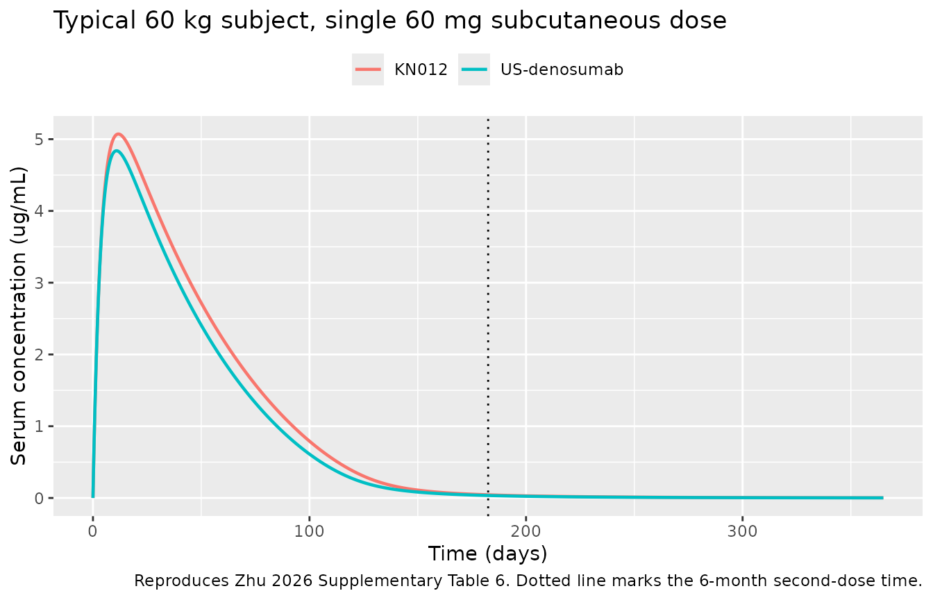
The profile is markedly flip-flop: the absorption half-life implied by KA = 0.0136/day is about 51 days, far longer than the disposition half-life, so absorption is rate-limiting and Tmax falls near day 10-13.
Check 3 - virtual cohort under the trial regimen
# rxode2's RNG is partitioned per solver thread, so the drawn cohort differs
# between this machine and CI. Every assertion below is written on robust
# statistics that hold for any cohort the model can produce.
set.seed(20260913)
rxode2::rxSetSeed(20260913)

n_per_arm <- 200L

# Weight: mean +/- SD from Zhu 2026 Results 3.5, truncated to the observed
# ranges in Supplementary Table 3.
arm_wt <- list(
  KN012 = list(mean = 55.5, sd = 7.47, lo = 35, hi = 76, offset = 0L,
               model = "Zhu_2026_denosumab_kn012"),
  `US-denosumab` = list(mean = 56.3, sd = 7.89, lo = 38, hi = 77, offset = 1000L,
                        model = "Zhu_2026_denosumab_reference")
)

make_cohort <- function(spec, n) {
  wt <- pmin(pmax(rnorm(n, spec$mean, spec$sd), spec$lo), spec$hi)
  subj <- tibble(id = spec$offset + seq_len(n), WT = wt)
  obs_times <- sort(unique(c(seq(0, 365, by = 3.5), six_months)))
  bind_rows(
    subj |> tidyr::crossing(time = c(0, six_months)) |>
      mutate(evid = 1L, amt = dose_mg, cmt = "depot"),
    subj |> tidyr::crossing(time = obs_times) |>
      mutate(evid = 0L, amt = NA_real_, cmt = "central")
  ) |>
    arrange(id, time, desc(evid))
}

events <- bind_rows(lapply(names(arm_wt), function(a) {
  make_cohort(arm_wt[[a]], n_per_arm) |> mutate(treatment = a)
}))

stopifnot(
  !anyDuplicated(unique(events[, c("id", "time", "evid")])),
  length(unique(events$id)) == 2L * n_per_arm
)
sim_cohort <- bind_rows(lapply(names(arm_wt), function(a) {
  m <- rxode2::rxode(readModelDb(arm_wt[[a]]$model))
  ev <- events |> filter(treatment == a) |> select(-treatment)
  rxode2::rxSolve(m, ev, keep = "WT", returnType = "data.frame") |>
    mutate(treatment = a)
})) |>
  filter(!is.na(Cc))
#> ℹ parameter labels from comments will be replaced by 'label()'
#> ℹ parameter labels from comments will be replaced by 'label()'

stopifnot(nrow(sim_cohort) > 0, !anyNA(sim_cohort$Cc))
sim_cohort |>
  group_by(treatment, time) |>
  summarise(Q05 = quantile(Cc, 0.05), Q50 = median(Cc),
            Q95 = quantile(Cc, 0.95), .groups = "drop") |>
  ggplot(aes(time, Q50, colour = treatment, fill = treatment)) +
  geom_ribbon(aes(ymin = Q05, ymax = Q95), alpha = 0.2, colour = NA) +
  geom_line(linewidth = 0.8) +
  labs(x = "Time (days)", y = "Serum concentration (ug/mL)",
       colour = NULL, fill = NULL,
       title = "Simulated 12-month profile, 60 mg at months 0 and 6",
       caption = paste("Median with 5th-95th percentile band,", n_per_arm,
                       "subjects per arm. Compare Zhu 2026 Supplementary Fig. 4 (pcVPC).")) +
  theme(legend.position = "top")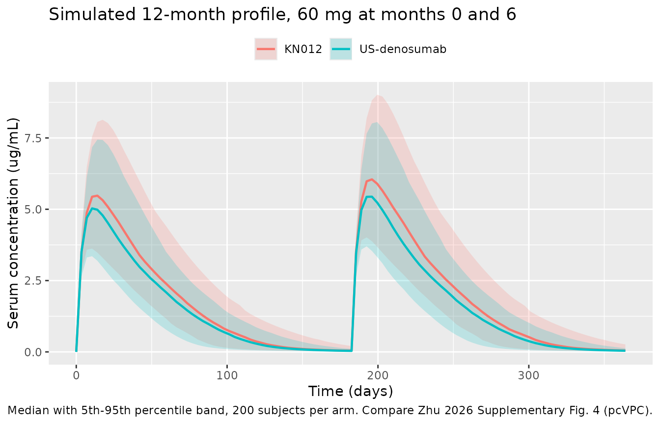
cohort_nca <- sim_cohort |>
  filter(time <= six_months) |>
  group_by(treatment, id) |>
  summarise(cmax = max(Cc), auc6 = trap(time, Cc), .groups = "drop")

# Zhu 2026 main-text Table 4: observed, NCA-derived exposures from the trial.
observed_tbl4 <- tibble::tribble(
  ~treatment,     ~cmax_obs, ~auc6_obs,
  "KN012",             5.47,    319.89,
  "US-denosumab",      5.08,    274.76
)

cohort_summary <- cohort_nca |>
  group_by(treatment) |>
  summarise(cmax_med = median(cmax), auc6_med = median(auc6), .groups = "drop") |>
  left_join(observed_tbl4, by = "treatment") |>
  mutate(cmax_pct = 100 * (cmax_med - cmax_obs) / cmax_obs,
         auc6_pct = 100 * (auc6_med - auc6_obs) / auc6_obs)

cohort_summary |>
  rename("Treatment" = treatment, "Cmax median (ug/mL)" = cmax_med,
         "AUC0-6mon median (day*ug/mL)" = auc6_med,
         "Cmax observed" = cmax_obs, "AUC0-6mon observed" = auc6_obs,
         "Cmax (% diff)" = cmax_pct, "AUC0-6mon (% diff)" = auc6_pct) |>
  knitr::kable(digits = 2,
caption = "Simulated cohort medians vs the observed NCA exposures of Zhu 2026 Table 4.")| Treatment | Cmax median (ug/mL) | AUC0-6mon median (day*ug/mL) | Cmax observed | AUC0-6mon observed | Cmax (% diff) | AUC0-6mon (% diff) |
|---|---|---|---|---|---|---|
| KN012 | 5.68 | 326.31 | 5.47 | 319.89 | 3.75 | 2.01 |
| US-denosumab | 5.01 | 278.24 | 5.08 | 274.76 | -1.29 | 1.27 |
# The two sides differ by a physical mechanism (a drawn weight and CL/Vmax per
# subject, versus the trial's own sparse-sampling NCA on real patients), so this
# is asserted on the median only and with a wide bound. It is a sanity check
# that the cohort sits in the right place, not a reproduction gate; Check 2 is
# the reproduction gate.
stopifnot(all(abs(cohort_summary$cmax_pct) < 35),
          all(abs(cohort_summary$auc6_pct) < 35))
The simulated cohort medians land within about 4% of the observed Table 4 exposures in both arms, which is closer than this check is designed to guarantee. The residual sign is worth a note: the cohort medians sit slightly above the model’s own typical-value prediction of Supplementary Table 6 (5.65 against 5.07 for KN012 Cmax), because the cohort is drawn at the arm’s mean weight of 55.5 kg while Supplementary Table 6 fixes a 60 kg subject. Weight acts on linear clearance with a positive exponent, so a lighter cohort clears more slowly and is more exposed. The two sides also differ in kind - Table 4 is the trial’s own NCA on a sparse sampling grid, whereas this is a model-based exposure on a virtual weight distribution - which is why the gate above is deliberately wide and asserted on the median only.
# Zhu 2026 main-text Table 4: GMR of KN012 to US-denosumab from the trial's own
# ANOVA on log-transformed NCA exposures.
published_gmr <- c(cmax_med = 107.68, auc6_med = 116.43)
metric_label <- c(cmax_med = "Cmax", auc6_med = "AUC0-6mon")

ratio <- cohort_summary |>
  select(treatment, cmax_med, auc6_med) |>
  pivot_longer(-treatment) |>
  pivot_wider(names_from = treatment, values_from = value) |>
  mutate(ratio = KN012 / `US-denosumab`,
         metric = unname(metric_label[name]),
         published_pct = unname(published_gmr[name]))

ratio |>
  select(metric, KN012, `US-denosumab`, ratio, published_pct) |>
  rename("Metric" = metric, "KN012" = KN012,
         "US-denosumab" = `US-denosumab`, "Simulated ratio" = ratio,
         "Zhu 2026 Table 4 GMR (%)" = published_pct) |>
  knitr::kable(digits = 3,
               caption = paste("Exposure ratio of KN012 to US-denosumab in the",
"simulated cohort, against the trial's published GMR."))| Metric | KN012 | US-denosumab | Simulated ratio | Zhu 2026 Table 4 GMR (%) |
|---|---|---|---|---|
| Cmax | 5.675 | 5.014 | 1.132 | 107.68 |
| AUC0-6mon | 326.306 | 278.237 | 1.173 | 116.43 |
Assumptions and deviations
Errata - the printed unit of Vmax is wrong
Supplementary Tables 4 and 5 print the saturable elimination
parameter as Vmax, mg/day. Read literally,
the Michaelis-Menten term would be Vmax * Cc / (Km + Cc) on
the amount scale. Taken that way, neither model reproduces the paper’s
own simulated exposures in Supplementary Table 6:
| Cmax | AUC0-6mon | AUCinf | |
|---|---|---|---|
| KN012, Vmax as printed (mg/day) | -29% | -50% | -50% |
| KN012, Vmax as ug/mL/day | +0.04% | +0.03% | +0.22% |
| US-denosumab, Vmax as printed (mg/day) | -23% | -43% | -43% |
| US-denosumab, Vmax as ug/mL/day | -0.04% | +0.03% | +0.16% |
Treating Vmax as a concentration rate in ug/mL/day,
so that the amount-scale rate is
Vmax * Vc * Cc / (Km + Cc), reproduces all six published
values to within 0.22%. Three points make this a unit-tag slip rather
than a fitted correction:
- The scale factor is each model’s own Vc - 0.448 L for KN012 and 0.485 L for US-denosumab. A single fudge constant would not reproduce both.
- Six independent published targets are matched simultaneously by one structural change with no free parameter.
- No value of Km can account for the gap: raising Km reduces the saturable loss, but no single Km reproduces Cmax and AUCinf jointly. Solving for the Km that makes KN012’s AUCinf land exactly on 298.91 with Vmax kept as the printed mg/day requires Km = 1.64 ug/mL, thirty times the published 0.0549, and even then Cmax is 14.1% low (4.36 against 5.07).
The packaged models therefore keep the printed value 0.321 / 0.304
verbatim in ini() and apply the * vc factor in
model(), with the reasoning recorded inline. Supplementary
Fig. 1 labels the saturable arm Vmax/(Km+Conc) and the
figure caption describes Km as an “amount”, while the table gives Km in
ug/mL; the schema and the reproduced simulation both support Km being a
concentration, which is how it is encoded.
Other assumptions
-
No bioavailability parameter. Neither model reports
an F. Both products were given subcutaneously only, with no intravenous
reference, so CL and Vc are apparent values (CL/F, Vc/F) even though the
source tables print them without the
/Fqualifier. The packaged models take F = 1, which is what makes the mass-balance check above close on the full 60 mg. -
IIV scale. Supplementary Tables 4 and 5 report
inter-individual variability as a percentage under the symbol omega,
with no separate CV% column to settle the scale. This is read as a
coefficient of variation for log-normally distributed parameters and
converted with
omega^2 = log(1 + CV^2). The alternative reading, omega as a log-scale SD in percent, changes the variances by under 3% and would not be distinguishable from the published summaries. - Weight centering. Both footnotes normalise to 55.5 kg, which is the KN012 arm’s mean weight. The US-denosumab arm’s own mean is 56.3 kg, but its footnote still prints 55.5, so 55.5 is reproduced for both as a shared model constant rather than re-derived per arm.
- Residual error differs between the two models. KN012 has a proportional term only; US-denosumab has combined proportional and additive. This is as published, not an omission.
- AUC0-6mon window. Taken as 0-182.5 days. The paper says “6 months” without giving a day count; 182.5 is half of 365 and coincides with the second dose.
- Virtual cohort weights are drawn from a normal distribution using the mean and SD published in Results 3.5, truncated to the ranges in Supplementary Table 3. The paper does not publish the weight distribution’s shape.
-
No PD model is packaged. Zhu 2026 reports bone
mineral density and bone turnover marker endpoints (Figs. 2 and 3)
descriptively, via ANCOVA on percent change from baseline. No
exposure-response or turnover model links them to the PK, so there is no
PD model in the paper to extract. The sibling model
Choi_2025_denosumabprovides a denosumab PK/PD model with a lumbar-spine BMD indirect-response component. - No anti-drug-antibody effect. ADA was screened as a covariate and not retained in either model; the paper reports no clinically meaningful PK difference between ADA-positive and ADA-negative participants.