Doxycycline rabbit (Mileva 2021)
Source:vignettes/articles/Mileva_2021_doxycycline_rabbit.Rmd
Mileva_2021_doxycycline_rabbit.RmdModel and source
- Citation: Mileva R, Rusenov A, Milanova A. Population Pharmacokinetic Modelling of Orally Administered Doxycycline to Rabbits at Different Ages. Antibiotics (Basel). 2021;10(3):310. doi:10.3390/antibiotics10030310
- Description: Preclinical (rabbit). One-compartment population PK model with first-order absorption and elimination for doxycycline hyclate given as a single 5 mg/kg oral dose in hard gelatin capsules to mature (5-month-old) and immature (70-day-old) New Zealand x Californian broiler rabbits, parameterised per kg body weight with no covariates (Mileva 2021)
- Article: https://doi.org/10.3390/antibiotics10030310 (open access)
- Supplement (Tables S1-S2): https://www.mdpi.com/2079-6382/10/3/310/s1
Mileva et al. gave a single oral dose of doxycycline hyclate (5 mg/kg, powder weighed into a hard gelatin capsule) to mature and immature rabbits and fitted a one-compartment model with first-order absorption and elimination in Phoenix NLME 8.3 (FOCE-ELS). Body weight, age and the pre-dose biochemistry (total protein, albumin, ALT, AST, LDH) were screened as covariates and none was retained, so the final model has no covariates. All structural parameters are per kg body weight and apparent (V/F, CL/F), because no intravenous reference was given.
Population
Eighteen clinically healthy crossbred New Zealand x Californian broiler rabbits were enrolled (Methods section 4.2): six mature 5-month-old animals (3.55 +/- 0.30 kg) and twelve immature 70-day-old animals (2.03 +/- 0.21 kg). Two immature rabbits expelled a damaged capsule and were excluded, leaving 16 animals (6 mature, 10 immature) in the analysis. Mature rabbits were sampled at 0.5, 1, 2, 3, 4, 6, 8, 10, 12 and 24 h; the immature animals were split into two sub-groups sampled at 0.5, 2, 4, 8, 12 h or at 1, 3, 6, 10, 24 h (Methods section 4.3). Free plasma doxycycline was measured by HPLC-PDA after TFA protein precipitation (LOQ 0.15 ug/mL); samples below the LOQ were not used in the fit. Sex was not reported.
The same information is available programmatically via
readModelDb("Mileva_2021_doxycycline_rabbit")()$population.
Source trace
| Equation / parameter | Value | Source location |
|---|---|---|
lka (ka) |
log(0.257) 1/h | Table 1, tvka
|
lcl (CL/F per kg) |
log(1.473) L/kg/h | Table 1, tVCl
|
lvc (V/F per kg) |
log(4.429) L/kg | Table 1, tvV
|
etalka |
0.103 | Table 2, variance of eta ka (BSV 32.96%) |
etalcl |
0.033 | Table 2, variance of eta Cl (BSV 18.18%) |
etalvc |
0.392 | Table 2, variance of eta V (BSV 69.30%) |
propSd |
0.368 | Table 1, stdev0; multiplicative error
Ct = f(theta, Time) x (1 + epsilon), Equation 8 |
P_i = tvP x exp(eta_i) |
n/a | Equation 5 (stated for V; “the other two parameters were calculated with the same algorithm”) |
| One compartment, first-order absorption and elimination | n/a | Results section 2; Methods section 4.5 |
kel = cl / vc |
n/a | Equation 2 (k10 = tvCl/tvV) |
| No covariates | n/a | Results section 2; Methods section 4.5 (“a model without covariates was chosen”) |
Dose 5 mg/kg into depot
|
n/a | Methods section 4.1 and 4.3 |
The paper’s own secondary parameters are internally consistent with
the primary estimates, which cross-checks the transcription:
k10 = 1.473 / 4.429 = 0.3326 1/h (Table 1: 0.332),
t1/2 = log(2) / k10 = 2.084 h (Table 1: 2.09),
AUC = Dose / CL = 5 / 1.473 = 3.394 ug*h/mL (Table 1:
3.40), and 100 x sqrt(exp(omega^2) - 1) returns the printed
BSV of 32.96% and 69.30% for ka and V (Equation 6). For CL it gives
18.3% against the printed 18.18%, which corresponds to an unrounded
variance of about 0.0325 printed as 0.033.
Typical-value checks
mod <- readModelDb("Mileva_2021_doxycycline_rabbit")
mod_typical <- rxode2::zeroRe(mod)
#> ℹ parameter labels from comments will be replaced by 'label()'

dose <- 5 # mg/kg
ka <- 0.257
cl <- 1.473
vc <- 4.429
kel <- cl / vc

ev_typ <- rxode2::et(amt = dose, cmt = "depot") |>
  rxode2::et(c(seq(0, 12, by = 0.05), seq(12.5, 48, by = 0.5)))
sim_typ <- rxode2::rxSolve(
  mod_typical,
  events = ev_typ,
  rtol = 1e-10,
  atol = 1e-12
) |>
  as.data.frame()
#> ℹ omega/sigma items treated as zero: 'etalka', 'etalcl', 'etalvc'

# Closed-form one-compartment oral solution with the same parameters.
closed_form <- dose / vc * ka / (ka - kel) *
  (exp(-kel * sim_typ$time) - exp(-ka * sim_typ$time))
stopifnot(max(abs(sim_typ$Cc - closed_form)) < 1e-6 * max(closed_form))

# Secondary parameters of Table 1 and the typical time of the peak.
tmax_typ <- log(ka / kel) / (ka - kel)
typical_checks <- tibble::tribble(
  ~Quantity, ~Model, ~Published,
  "k10 (1/h)", kel, 0.332,
  "Half-life log(2)/k10 (h)", log(2) / kel, 2.09,
  "AUC0-inf = Dose/CL (ug*h/mL)", dose / cl, 3.40
) |>
  mutate(`% diff` = 100 * (Model / Published - 1))
knitr::kable(
  typical_checks,
  digits = c(0, 3, 3, 2),
  caption = "Table 1 secondary parameters recomputed from the packaged typical values."
)| Quantity | Model | Published | % diff |
|---|---|---|---|
| k10 (1/h) | 0.333 | 0.332 | 0.17 |
| Half-life log(2)/k10 (h) | 2.084 | 2.090 | -0.28 |
| AUC0-inf = Dose/CL (ug*h/mL) | 3.394 | 3.400 | -0.16 |
The typical profile peaks at 3.41 h at 0.363 ug/mL. Because
ka (0.257 1/h) is smaller than k10 (0.333
1/h), the model is in flip-flop: the terminal slope of the
concentration-time curve is set by absorption, so the terminal half-life
is log(2) / ka = 2.7 h, not the 2.09 h k10
half-life reported in Table 1. The PKNCA half-life below therefore sits
near 2.7 h.
Virtual cohort and simulation
Each simulated animal receives 5 mg/kg into depot and is
observed on the study’s sampling schedule. Because the final model has
no covariates, the mature and immature arms differ only in their
sampling design: 200 mature animals sampled at all ten times, and 200
immature animals split into the two sampling sub-groups. As in the
paper, samples below the 0.15 ug/mL LOQ are removed before the
observed-style summaries.
set.seed(2021)
rxode2::rxSetSeed(2021)

make_cohort <- function(n, times, group, id_offset) {
  ids <- id_offset + seq_len(n)
  doses <- tibble(
    id = ids,
    time = 0,
    amt = dose,
    evid = 1L,
    cmt = "depot",
    group = group
  )
  obs <- tidyr::expand_grid(id = ids, time = times) |>
    mutate(amt = 0, evid = 0L, cmt = "central", group = group)
  bind_rows(doses, obs) |>
    arrange(id, time, desc(evid))
}

events <- bind_rows(
  make_cohort(200, c(0.5, 1, 2, 3, 4, 6, 8, 10, 12, 24), "Mature", 0L),
  make_cohort(100, c(0.5, 2, 4, 8, 12), "Immature", 200L),
  make_cohort(100, c(1, 3, 6, 10, 24), "Immature", 300L)
)
stopifnot(!anyDuplicated(unique(events[, c("id", "time", "evid")])))

sim <- rxode2::rxSolve(mod, events = events, keep = "group") |>
  as.data.frame()
#> ℹ parameter labels from comments will be replaced by 'label()'

# `sim` carries the residual-error draw (the observation); `Cc` is the
# individual prediction.
loq <- 0.15
sim_obs <- sim |>
  filter(time > 0) |>
  rename(Cobs = sim)
Replicate published figures
Supplementary Table S1 gives the observed mean +/- SD concentration per age group; the 12-h mature value is the mean of the quantifiable samples only.
observed <- tibble::tribble(
  ~time, ~Mature, ~Immature,
  0.5, 0.17, 0.25,
  1, 0.22, 0.42,
  2, 0.27, 0.36,
  3, 0.35, 0.45,
  4, 0.56, 0.73,
  6, 0.25, 0.33,
  8, 0.17, 0.26,
  10, 0.18, 0.20,
  12, 0.13, 0.17
) |>
  pivot_longer(-time, names_to = "group", values_to = "mean_obs")
# Replicates Figure 1b of Mileva 2021: VPC with 10th, 50th and 90th
# percentiles of simulated observations over 0-12 h (both age groups pooled,
# as in the paper).
vpc <- sim_obs |>
  filter(time <= 12) |>
  group_by(time) |>
  summarise(
    p10 = quantile(Cobs, 0.10),
    p50 = quantile(Cobs, 0.50),
    p90 = quantile(Cobs, 0.90),
    .groups = "drop"
  )

ggplot(vpc, aes(time)) +
  geom_ribbon(aes(ymin = p10, ymax = p90), alpha = 0.25, fill = "steelblue") +
  geom_line(aes(y = p50), colour = "steelblue4") +
  geom_point(
    data = observed,
    aes(y = mean_obs, shape = group),
    colour = "firebrick"
  ) +
  geom_hline(yintercept = loq, linetype = "dotted") +
  scale_y_log10() +
  labs(
    x = "Time (h)",
    y = "Doxycycline (ug/mL)",
    shape = "Observed mean (Table S1)",
    title = "Simulated 10th-50th-90th percentiles after 5 mg/kg orally",
    caption = "Replicates Figure 1b of Mileva 2021; dotted line = LOQ."
  )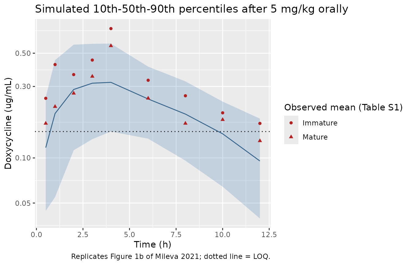
The paper’s Figure 1b predicted median, read from the figure by the maintainers, is about 0.34 ug/mL at 3.5 h and 0.10 ug/mL at 12 h.
fig1b_median <- tibble::tribble(
  ~time, ~digitised,
  3.5, 0.34,
  12, 0.10
)
typ_at <- approx(sim_typ$time, sim_typ$Cc, xout = fig1b_median$time)$y
fig1b_median <- fig1b_median |>
  mutate(typical = typ_at, pct_diff = 100 * (typical / digitised - 1))
knitr::kable(
  fig1b_median,
  digits = c(1, 2, 3, 1),
  caption = "Typical-value prediction vs the predicted median read from Figure 1b."
)| time | digitised | typical | pct_diff |
|---|---|---|---|
| 3.5 | 0.34 | 0.363 | 6.7 |
| 12.0 | 0.10 | 0.105 | 4.8 |
# The digitised values are read by eye from a log axis (about 10% reading
# error); 20% still fails for a two-fold error in V/F, CL/F or the dose.
stopifnot(all(abs(fig1b_median$pct_diff) < 20))
The simulated median follows the paper’s predicted median closely. The simulated 10th-90th percentile band (about 0.11-0.58 ug/mL at 2-4 h) also agrees with the paper’s observed 10th and 90th percentiles in Figure 1b (about 0.12-0.16 and 0.4-0.8 ug/mL). It is, however, much narrower than the paper’s predicted 10th and 90th percentiles, which in Figure 1b reach about 1.1-1.6 ug/mL at the top and fall to about 0.002-0.005 ug/mL at 10-12 h at the bottom. Those bands cannot be produced from the variances printed in Tables 1 and 2, whose internal consistency is shown above; see Assumptions and deviations.
PKNCA validation
Two NCA runs feed one comparison table. The typical value row uses the deterministic typical profile and compares against the Table 1 secondary parameters. The Mature and Immature rows use the simulated observations (residual error included, samples below LOQ removed) on the study’s sampling schedule and compare against the observed Cmax and Tmax the paper reports in Results section 2.
# Typical-value profile. Concentrations decayed into solver noise are floored
# (pattern: a negative undershoot of order atol would make PKNCA return NaN).
stopifnot(all(sim_typ$Cc >= -1e-6 * max(sim_typ$Cc)))
typ_conc <- sim_typ |>
  filter(!is.na(Cc)) |>
  mutate(Cc = pmax(Cc, 0), id = 1L, treatment = "Typical value") |>
  select(id, time, Cc, treatment)
typ_dose <- tibble(id = 1L, time = 0, amt = dose, treatment = "Typical value")
typ_nca <- PKNCA::pk.nca(PKNCA::PKNCAdata(
  PKNCA::PKNCAconc(typ_conc, Cc ~ time | treatment + id),
  PKNCA::PKNCAdose(typ_dose, amt ~ time | treatment + id),
  intervals = data.frame(
    start = 0,
    end = Inf,
    aucinf.obs = TRUE,
    half.life = TRUE
  )
))

# Observed-style cohort: quantifiable simulated observations only.
coh_conc <- sim_obs |>
  mutate(Cobs = if_else(Cobs >= loq, Cobs, NA_real_)) |>
  filter(!is.na(Cobs)) |>
  transmute(id, time, Cc = Cobs, treatment = group)
coh_conc <- bind_rows(
  coh_conc,
  coh_conc |> distinct(id, treatment) |> mutate(time = 0, Cc = 0)
) |>
  distinct(id, treatment, time, .keep_all = TRUE) |>
  arrange(id, treatment, time)
coh_dose <- events |>
  filter(evid == 1, id %in% coh_conc$id) |>
  transmute(id, time, amt, treatment = group)
coh_nca <- PKNCA::pk.nca(PKNCA::PKNCAdata(
  PKNCA::PKNCAconc(coh_conc, Cc ~ time | treatment + id),
  PKNCA::PKNCAdose(coh_dose, amt ~ time | treatment + id),
  intervals = data.frame(start = 0, end = 24, cmax = TRUE, tmax = TRUE)
))

nca_long <- bind_rows(
  as.data.frame(typ_nca$result),
  as.data.frame(coh_nca$result)
) |>
  select(treatment, PPTESTCD, PPORRES)
published <- tibble::tribble(
  ~treatment, ~cmax, ~tmax, ~aucinf.obs, ~half.life,
  "Typical value", NA, NA, 3.40, 2.09,
  "Mature", 0.58, 3.40, NA, NA,
  "Immature", 0.60, 3.63, NA, NA
)

# Compare only the (group, parameter) pairs the paper reports.
published_long <- published |>
  pivot_longer(-treatment, names_to = "PPTESTCD", values_to = "PPORRES") |>
  filter(!is.na(PPORRES))
stopifnot(nrow(published_long) == 6L)

cmp <- nlmixr2lib::ncaComparisonTable(
  simulated = semi_join(nca_long, published_long, by = c("treatment", "PPTESTCD")),
  reference = published_long,
  by = "treatment",
  params = c("cmax", "tmax", "aucinf.obs", "half.life"),
  units = c(
    cmax = "ug/mL",
    tmax = "h",
    aucinf.obs = "ug*h/mL",
    half.life = "h"
  ),
  tolerance_pct = 20
)
stopifnot(nrow(cmp) == 6L)
knitr::kable(
  cmp,
  caption = paste(
    "Simulated (median across animals) vs published NCA.",
    "* differs from the reference by >20%.",
    "Published Cmax and Tmax are the observed means (Results section 2);",
    "published AUC and half-life are the Table 1 secondary parameters."
  )
)| NCA parameter | treatment | Reference | Simulated | % diff |
|---|---|---|---|---|
| Cmax (ug/mL) | Mature | 0.58 | 0.419 | -27.7%* |
| Cmax (ug/mL) | Immature | 0.6 | 0.382 | -36.3%* |
| Tmax (h) | Mature | 3.4 | 4 | +17.6% |
| Tmax (h) | Immature | 3.63 | 4 | +10.2% |
| AUC0-∞ (obs) (ug*h/mL) | Typical value | 3.4 | 3.39 | -0.2% |
| t½ (h) | Typical value | 2.09 | 2.78 | +33.0%* |
nca_val <- function(grp, code) {
  v <- nca_long$PPORRES[nca_long$treatment == grp & nca_long$PPTESTCD == code]
  if (length(v) == 1L) {
    return(v)
  }
  v <- v[!is.na(v)]
  if (length(v) == 0L) {
    stop("no NCA value for ", grp, " / ", code)
  }
  median(v)
}
auc_typ <- nca_val("Typical value", "aucinf.obs")
hl_typ <- nca_val("Typical value", "half.life")
cmax_mat <- nca_val("Mature", "cmax")
cmax_imm <- nca_val("Immature", "cmax")
tmax_mat <- nca_val("Mature", "tmax")
tmax_imm <- nca_val("Immature", "tmax")

stopifnot(
  # Deterministic: AUC0-inf of the typical profile is Dose/CL (Table 1).
  abs(auc_typ / 3.40 - 1) < 0.01,
  # Deterministic: terminal half-life is absorption-limited (flip-flop).
  # PKNCA's best-fit window starts near 19 h, where the k10 exponential still
  # contributes a little, so it returns about 2.78 h against log(2)/ka = 2.70 h;
  # the k10 half-life (2.09 h) is far outside this bound.
  abs(hl_typ / (log(2) / ka) - 1) < 0.05,
  # Cohort medians (robust to which animals land in the tails): Tmax sits on
  # the 3-4 h sampling times, and Cmax is within a factor of two of the
  # observed means. A two-fold error in V/F or the dose breaks the Cmax bound.
  tmax_mat >= 2, tmax_mat <= 6,
  tmax_imm >= 2, tmax_imm <= 6,
  cmax_mat > 0.29, cmax_mat < 1.16,
  cmax_imm > 0.30, cmax_imm < 1.20
)
AUC0-inf reproduces Table 1 exactly. The half-life row
is starred by design: Table 1 reports the k10 half-life,
whereas PKNCA estimates the terminal half-life, which here is the
absorption half-life (flip-flop, see above).
The simulated median Cmax is 28% (mature) and 36% (immature) below
the observed mean Cmax. The Table S1 means show a sharp peak at 4 h
(0.56 and 0.73 ug/mL) between 0.35-0.45 ug/mL at 3 h and 0.25-0.33 ug/mL
at 6 h, a shape a one-compartment model with a slow first-order
absorption (ka < k10) cannot reproduce; the
paper’s own predicted median in Figure 1b (about 0.34 ug/mL at the peak)
and its Figure 1a individual curves (mostly below 0.5 ug/mL) show the
same under-prediction of the peak. This is a property of the published
model, not of the transcription; the parameters were not adjusted.
%fT > MIC
The paper reports that a 5 mg/kg dose gives %fT > MIC of 35% for
an assumed MIC of 0.18 ug/mL and a 12-h dosing interval, using Equation
9, %fT>MIC = ln(Cmax / MIC) x (1 / k10) x 100 / tau.
That value is reproduced exactly when the Cmax entered is the highest
observed mean concentration in Table S1 (0.73 ug/mL, immature rabbits at
4 h), which appears to be the value the authors used.
mic <- 0.18
tau <- 12
ftmic_eq9 <- function(cmax) log(cmax / mic) / 0.332 * 100 / tau
ftmic <- tibble::tribble(
  ~`Cmax used`, ~Cmax,
  "Highest Table S1 mean (immature, 4 h)", 0.73,
  "Observed mean Cmax, mature (Results)", 0.58,
  "Observed mean Cmax, immature (Results)", 0.60,
  "Typical-value model Cmax", max(sim_typ$Cc)
) |>
  mutate(`%fT>MIC (Equation 9)` = ftmic_eq9(Cmax))

# Time above MIC from the typical-value profile itself (single dose, 0-12 h).
above <- sim_typ |> filter(time <= tau)
pct_above_typ <- 100 * mean(above$Cc > mic)
knitr::kable(
  ftmic,
  digits = c(0, 3, 1),
  caption = "Equation 9 of Mileva 2021 evaluated at different Cmax values."
)| Cmax used | Cmax | %fT>MIC (Equation 9) |
|---|---|---|
| Highest Table S1 mean (immature, 4 h) | 0.730 | 35.1 |
| Observed mean Cmax, mature (Results) | 0.580 | 29.4 |
| Observed mean Cmax, immature (Results) | 0.600 | 30.2 |
| Typical-value model Cmax | 0.363 | 17.6 |
Equation 9 assumes an intravenous-bolus-like decline from Cmax. Read directly from the typical-value profile, the single-dose concentration stays above 0.18 ug/mL for about 70% of the first 12 h, because the slow absorption keeps the profile near its plateau for several hours.
Assumptions and deviations
- Per-kg dosing. Dose (mg/kg), V/F (L/kg) and CL/F (L/kg/h) are kept per kg body weight exactly as published; enter the dose in mg/kg. Whole-animal V/F and CL/F are proportional to body weight, which was screened as a covariate and not retained.
-
Residual error unit. Table 1 lists
stdev0 = 0.368with the unit “ug/mL”, but its footnote and Equation 8 (Ct = f(theta, Time) x (1 + epsilon)) define it as the standard deviation of a multiplicative error, so it is dimensionless and is encoded aspropSd = 0.368. - IIV structure. Equation 5 is exponential BSV on V, with ka and CL “calculated with the same algorithm”. Table 2 lists only the three variances, so the omega matrix is diagonal.
- Figure 1b prediction interval. The paper’s predicted 10th and 90th percentile bands are much wider than a simulation from Tables 1 and 2 gives (and wider than the paper’s own observed 10th and 90th percentiles). The printed estimates are self-consistent (k10, half-life, AUC and the BSV percentages all recompute from them), so the tables were used as printed and only the predicted median of Figure 1b is used as a check. The cause of the wide published band is not stated.
- Peak under-prediction. The model under-predicts the observed mean Cmax by roughly 25-40% (see the NCA table); this is inherent to the published one-compartment model and is visible in the paper’s own figures.
-
Screened covariates. Body weight, age, total
protein, albumin, ALT, AST and LDH were tested and not retained; they
are recorded in
covariatesDataExcludedfor provenance. The paper does not state which parameter each covariate was tested on. - Sampling footnote. The Table S1 footnote says six immature rabbits were sampled at each time, whereas Methods section 4.3 describes two sub-groups of five; the simulation follows the Methods.
- Errata. No correction notice for this article was found on Europe PMC or the publisher’s page as of 2026-09-28.