Midazolam (Voller 2019)
Source:vignettes/articles/Voller_2019_midazolam.Rmd
Voller_2019_midazolam.RmdModel and source
- Citation: Voller S, Flint RB, Beggah F, Reiss I, Andriessen P, Zimmermann LJI, van den Anker JN, Liem KD, Koch BCP, de Wildt S, Knibbe CAJ, Simons SHP (2019). Recently Registered Midazolam Doses for Preterm Neonates Do Not Lead to Equal Exposure: A Population Pharmacokinetic Model. J Clin Pharmacol 59(10):1300-1308. doi:10.1002/jcph.1429.
- Description: One-compartment intravenous population PK model for midazolam in preterm neonates (55 neonates, gestational age 24.0-33.6 weeks, actual body weight 0.6-4.3 kg) pooled from the prospective multicentre DINO study and the de Wildt 1998 data set. Actual body weight enters clearance as a power function with an estimated exponent of 1.69 and central volume as a linear function (exponent fixed at 1), both centred on the 1.12 kg cohort median. The steeply supra-allometric clearance exponent reflects CYP3A maturation over the preterm weight range and is the basis of the paper’s finding that the registered flat 0.03 mg/(kg*h) infusion does not give equal exposure. No covariate other than actual body weight was retained.
- Article: J Clin Pharmacol 2019;59(10):1300-1308
Voller and colleagues pooled 232 midazolam plasma concentrations from 55 preterm neonates and fitted a one-compartment intravenous model in NONMEM 7.3. Their purpose was not the model for its own sake: a flat, weight-normalised infusion rate of 0.03 mg/(kg*h) had just been written into the midazolam label for neonates below 32 weeks of gestation, and they used the model to show that such a rate does not give equal exposure across the preterm weight range. It does not, because clearance rises with body weight far faster than proportionally – the estimated power exponent is 1.69, well above the allometric 0.75 and above even the isometric 1 – while the dose rises exactly proportionally. The lightest neonates are therefore over-exposed and the heaviest under-exposed on the same mg/(kg*h).
That structure makes this an unusually well-gated paper to validate against. Because clearance and volume both carry the covariate and nothing else does, the typical-value predictions are closed-form, and the paper prints enough of its own derived numbers – three steady-state-region concentrations, a nine-point dose-adjustment ladder, and six tail probabilities from its simulation – that essentially every element of the model can be checked against a published quantity rather than against itself.
Population
The analysis data set (Voller 2019 Table 1) combines two studies conducted in Dutch level III neonatal intensive care units.
Study 1 is the prospective multicentre Drug dosage Improvement NeOnates (DINO) study (MEC-2014-067, NL47409.078.14, NCT02421068), run from September 2014 to September 2017 in four centres. It contributed 29 neonates (13 female, 16 male) born before 32 weeks of gestation, with 60 sparse opportunistic samples drawn over follow-up periods of up to 30 days, and 123 intravenous doses – 59 short infusions of 30 minutes or less for stressful procedures and 65 continuous sedation infusions longer than 30 minutes, with the dose chosen by the treating physician. Median gestational age 26.7 weeks (range 24.0-31.1), median birth weight 0.84 kg (0.47-1.8), median actual body weight 1.3 kg (0.6-4.3), median postnatal age at inclusion 18 days (1-88).
Study 2 is the previously published de Wildt et al data set (MEC171.586/1998/125) from the Sophia Children’s Hospital, Rotterdam. It contributed 26 neonates (16 female, 10 male) each given a single 0.1 mg/kg intravenous dose over 30 minutes for a stressful procedure, densely sampled at 0.5, 1, 2, 4, 6, 12 and 24 hours – 172 concentrations in total. Median gestational age 28.1 weeks (26.3-33.6), median birth weight 1.1 kg (0.75-1.6), median actual body weight 1.0 kg (0.77-1.6), median postnatal age 5.5 days (3-11).
The combined set is 55 neonates, 232 samples and 149 doses; 29 of 55 (53%) were female, median gestational age 27.3 weeks (24.0-33.6) and median actual body weight 1.1 kg (0.6-4.3). The two studies used different assays – gas chromatography with mass spectrometric detection for study 2 (lower limit of quantification 1 ug/L) and liquid chromatography-tandem mass spectrometry for study 1 (lower limit of quantification 4 ug/L) – which the Discussion names as one likely contributor to the large unexplained between-subject variability. No target midazolam concentration has been established in this population; the 400 ug/L used throughout the paper is the indicative value proposed by Ahsman et al, being the median concentration those authors observed in term neonates whom they assumed had been successfully titrated to target sedation.
The same information is available programmatically from the model’s
population metadata
(readModelDb("Voller_2019_midazolam")()$population –
readModelDb() returns the model function, so the
trailing () evaluates it to the model object).
Source trace
The per-parameter origin is recorded as an in-file comment next to
each ini() entry in
inst/modeldb/specificDrugs/Voller_2019_midazolam.R. The
table below collects them in one place.
| Equation / parameter | Value | Source location |
|---|---|---|
lcl (CL at 1.12 kg) |
log(0.0737) L/h |
Table 2, row CL [L/h] = CL_p, final-model estimate
0.0737 (RSE 13%); restated in the Abstract as “73.7 mL/h for a neonate
weighing 1.1 kg” |
lvc (V at 1.12 kg) |
log(1.03) L |
Table 2, row V [L] = V_p, final-model estimate 1.03
(RSE 21%); restated in the Abstract as “1.03 L for a neonate weighing
1.1 kg” |
e_wt_cl |
1.69 | Table 2, row CL_i = CL_p x (WT_i/Median WT)^theta_WT,
theta_WT = 1.69 (RSE 10%); Results: power function of actual body weight
on CL, p < .001, -116 points in objective function value |
e_wt_vc |
fixed(1) |
Table 2 prints the volume row as
V_i = V_p x (WT_i/Median WT) with no exponent; Results: the
estimated volume exponent “was close to 1”, a linear form fitted equally
well (+0.2 points in objective function value) “and was therefore
carried forward” |
| Covariate centring, 1.12 kg | 1.12 kg | Table 2 footnote: “p, population mean value of a parameter for an individual with body weight of 1.12 kg … WT, actual body weight (median WT = 1.12 kg)” |
etalcl |
0.844561 (omega = 0.919) | Table 2, row On CL [%] = 91.9 (RSE 15%, eta shrinkage
8%); scale convention established below |
etalvc |
0.451584 (omega = 0.672) | Table 2, row On V [%] = 67.2 (RSE 16%, eta shrinkage
17%); scale convention established below |
propSd |
0.338 | Table 2, Residual variability, row Proportional (%) =
33.8 (RSE 16%) |
addSd |
0.218 ug/L | Table 2, Residual variability, row Additive (ug/L) =
0.218 (RSE 56%) |
d/dt(central) <- -kel * central |
n/a | Results: “A 1-compartment model described the available data best.” Both studies gave midazolam intravenously (bolus, short infusion, or continuous infusion), so there is no absorption state and no bioavailability term |
Cc <- central / vc |
n/a | Doses supplied in ug and volumes in L give ug/L, the unit used throughout the paper (target 400 ug/L, assay limits of quantification 1 and 4 ug/L) |
Cc ~ add(addSd) + prop(propSd) |
n/a | Table 2 reports both a proportional and an additive residual term |
Bootstrap estimates (1000 samples, 83.1% convergence) are reported alongside every final estimate in Table 2 and agree closely with them: CL 0.0787 (95%CI 0.0550-0.102), theta_WT 1.67 (0.406-2.47), V 1.11 (0.877-1.37), IIV on CL 96.6 (67.5-128), IIV on V 72.7 (47.4-96.8), proportional error 34.0 (28.6-39.4), additive error 0.283 (0.0800-0.585). The model file carries the final estimates, per the standing convention.
mod <- readModelDb("Voller_2019_midazolam")

# Published Table 2 constants, used by every gate below.
CL_REF  <- 0.0737 # L/h at the covariate-centring weight
V_REF   <- 1.03   # L at the covariate-centring weight
WT_REF  <- 1.12   # kg, Table 2 footnote
EXP_CL  <- 1.69   # power exponent of WT on CL
OM_CL   <- 0.919  # Table 2 'On CL [%]' / 100
OM_V    <- 0.672  # Table 2 'On V [%]'  / 100

cl_typ <- function(wt) CL_REF * (wt / WT_REF)^EXP_CL
v_typ  <- function(wt) V_REF * (wt / WT_REF)
Virtual cohort
The original data are not publicly available. Every simulation below uses the nine hypothetical body weights the paper itself simulated (Methods, “Evaluation of the Recently Registered Dosing Regimen”): 0.5, 0.75, 1, 1.25, 1.5, 1.75, 2, 2.25 and 2.5 kg. Body weight is the model’s only covariate, so a weight grid is a complete specification of the covariate distribution; nothing else has to be assumed.
Doses are supplied in ug to match the model’s declared
units (dosing = "ug"), so a rate of 0.03
mg/(kg*h) for a wt kg neonate is
0.03 * wt * 1000 ug/h.
WEIGHTS <- c(0.5, 0.75, 1, 1.25, 1.5, 1.75, 2, 2.25, 2.5)

# One arm per body weight. `n` subjects per arm; n = 1 with the random effects
# zeroed gives the typical-value profile. Doses target the `central` ODE state
# by name -- never the algebraic observable `Cc`, which would inject a new
# compartment slot and renumber the state vector.
make_infusion_events <- function(weights, n, rate_mgkgh, dur_h, obs_times,
                                 id_offset = 0L) {
  arms <- lapply(seq_along(weights), function(k) {
    wt <- weights[k]
    rate_ugh <- rate_mgkgh * wt * 1000
    ids <- id_offset + (k - 1L) * n + seq_len(n)
    dosing <- tibble(
      id = ids, time = 0, evid = 1L, cmt = "central",
      amt = rate_ugh * dur_h, rate = rate_ugh
    )
    obs <- tidyr::expand_grid(id = ids, time = obs_times) |>
      mutate(evid = 0L, cmt = "central", amt = NA_real_, rate = NA_real_)
    bind_rows(dosing, obs) |>
      mutate(WT = wt, treatment = sprintf("%.2f kg", wt))
  })
  bind_rows(arms) |> arrange(id, time, desc(evid))
}
Typical-value reproduction of the paper’s own derived numbers
The Results section prints three concentrations that the final model predicts 72 hours into a 0.03 mg/(kg*h) infusion: 754, 421 and 262 ug/L for neonates of 0.5, 1.25 and 2.5 kg. These are population predictions, so they are a direct, noise-free test of the structural model, the covariate functions, the centring weight and the unit convention all at once. A mis-transcribed exponent, a centring weight of 1.1 instead of 1.12, or a factor-of-1000 unit slip each move them by tens of percent.
obs_grid <- seq(0, 72, by = 0.5)

ev_typ <- make_infusion_events(WEIGHTS, n = 1L, rate_mgkgh = 0.03,
                               dur_h = 72, obs_times = obs_grid)

mod_typ <- mod |> rxode2::zeroRe()
#> ℹ parameter labels from comments will be replaced by 'label()'
sim_typ <- rxode2::rxSolve(mod_typ, events = ev_typ, keep = c("WT", "treatment"))
#> ℹ omega/sigma items treated as zero: 'etalcl', 'etalvc'
#> Warning: multi-subject simulation without without 'omega'

c72 <- as.data.frame(sim_typ) |>
  filter(abs(time - 72) < 1e-9) |>
  transmute(WT, treatment, Cc_sim = Cc)

published_c72 <- tibble(WT = c(0.5, 1.25, 2.5), Cc_pub = c(754, 421, 262))

chk_c72 <- c72 |>
  inner_join(published_c72, by = "WT") |>
  mutate(pct_diff = 100 * (Cc_sim - Cc_pub) / Cc_pub)

chk_c72 |>
  rename(
    "Body weight (kg)" = WT,
    "Simulated C(72 h) (ug/L)" = Cc_sim,
    "Published C(72 h) (ug/L)" = Cc_pub,
    "Difference (%)" = pct_diff
  ) |>
  select(-treatment) |>
  knitr::kable(
    digits = c(2, 1, 0, 2),
    caption = paste(
      "Population-predicted midazolam concentration 72 h into a",
      "0.03 mg/(kg*h) infusion, against the three values printed in the",
      "Voller 2019 Results section."
    )
)| Body weight (kg) | Simulated C(72 h) (ug/L) | Published C(72 h) (ug/L) | Difference (%) |
|---|---|---|---|
| 0.50 | 753.8 | 754 | -0.02 |
| 1.25 | 421.0 | 421 | 0.00 |
| 2.50 | 261.9 | 262 | -0.02 |
# Deterministic: zeroRe() removes every random effect, so this is the same
# closed-form quantity on both sides and no cohort noise can enter. The
# published values are rounded to 3 significant figures, which alone permits
# ~0.2%; 1% keeps headroom for that rounding while still failing loudly on any
# transcription error, which would move these by tens of percent.
stopifnot(max(abs(chk_c72$pct_diff)) < 1)
# Replicates Figure 3A of Voller 2019: population-predicted concentration-time
# profiles over 72 h at the labelled 0.03 mg/(kg*h) rate, with the indicative
# 400 ug/L target of Ahsman et al as a dashed line.
as.data.frame(sim_typ) |>
  mutate(treatment = factor(treatment, levels = sprintf("%.2f kg", WEIGHTS))) |>
  ggplot(aes(time, Cc, colour = treatment)) +
  geom_line(linewidth = 0.7) +
  geom_hline(yintercept = 400, linetype = "dashed") +
  scale_colour_viridis_d(name = "Body weight") +
  labs(
    x = "Time (h)", y = "Midazolam concentration (ug/L)",
    title = "Figure 3A - labelled 0.03 mg/(kg*h) infusion",
    caption = "Replicates Figure 3A of Voller 2019."
  ) +
  theme_bw()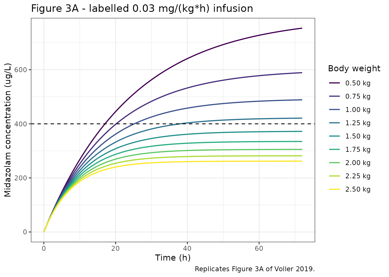
The ordering the paper emphasises is visible immediately: the lightest neonates sit highest. Because clearance scales as weight to the 1.69 while the infusion rate scales as weight to the 1, the steady-state concentration scales as weight to the -0.69, so halving body weight raises exposure by about 60%.
Time to steady state
The paper also reports that time to steady state differs by weight – reached after 24 hours at 2 kg or more, more than 48 hours at 1 kg or less. That reading is taken off Figure 3A and the paper states no numerical threshold for “steady state”, so the table below reports the times to 90% and 95% of the asymptote for reference and the gate is placed on the claim the paper actually makes structurally: that time to steady state falls monotonically with body weight.
# Elimination rate constant is closed-form for this model:
#   kel = CL/V = (0.0737/1.03) * (WT/1.12)^(1.69 - 1)
tss <- tibble(WT = WEIGHTS) |>
  mutate(
    kel = cl_typ(WT) / v_typ(WT),
    t90 = log(10) / kel,
    t95 = log(20) / kel
  )

tss |>
  rename(
    "Body weight (kg)" = WT,
    "kel (1/h)" = kel,
    "Time to 90% of Css (h)" = t90,
    "Time to 95% of Css (h)" = t95
  ) |>
  knitr::kable(
    digits = c(2, 4, 1, 1),
    caption = "Time to approach the steady-state asymptote by body weight."
)| Body weight (kg) | kel (1/h) | Time to 90% of Css (h) | Time to 95% of Css (h) |
|---|---|---|---|
| 0.50 | 0.0410 | 56.1 | 73.0 |
| 0.75 | 0.0543 | 42.4 | 55.2 |
| 1.00 | 0.0662 | 34.8 | 45.3 |
| 1.25 | 0.0772 | 29.8 | 38.8 |
| 1.50 | 0.0875 | 26.3 | 34.2 |
| 1.75 | 0.0974 | 23.7 | 30.8 |
| 2.00 | 0.1068 | 21.6 | 28.1 |
| 2.25 | 0.1158 | 19.9 | 25.9 |
| 2.50 | 0.1245 | 18.5 | 24.1 |
Figure 3B: the dose-adjustment ladder
Figure 3B and the accompanying Results text give the infusion rate needed at each body weight to bring the typical steady-state concentration to 400 ug/L within 10%: 0.015 mg/(kg*h) at 0.5 kg, 0.02 at 0.75 kg, 0.024 at 1 kg, the labelled 0.03 unchanged at 1.25 and 1.5 kg, 0.036 at 1.75 kg, 0.04 at 2 and 2.25 kg, and a 50% increase to 0.045 at 2.5 kg.
This is a nine-point test of the clearance-versus-weight function across the whole preterm range, and it is independent of the previous gate because it inverts the relationship rather than evaluating it. The published ladder is rounded to a prescribable rate, so the gate is the paper’s own criterion – each stated rate must put the typical steady-state concentration inside 400 ug/L +/- 10% – with the exact required rate reported alongside.
published_ladder <- tibble(
  WT = WEIGHTS,
  rate_pub = c(0.015, 0.020, 0.024, 0.030, 0.030, 0.036, 0.040, 0.040, 0.045)
)

ladder <- published_ladder |>
  mutate(
    CL = cl_typ(WT),
    Css_at_pub = rate_pub * WT * 1000 / CL,
    rate_exact = 400 * CL / (WT * 1000),
    in_band = Css_at_pub >= 360 & Css_at_pub <= 440
  )

ladder |>
  select(WT, rate_pub, Css_at_pub, rate_exact, in_band) |>
  rename(
    "Body weight (kg)" = WT,
    "Published rate (mg/(kg*h))" = rate_pub,
    "Typical Css at that rate (ug/L)" = Css_at_pub,
    "Exact rate for 400 ug/L (mg/(kg*h))" = rate_exact,
    "Within 400 +/- 10%" = in_band
  ) |>
  knitr::kable(
    digits = c(2, 3, 1, 4, 0),
    caption = paste(
      "Figure 3B dose-adjustment ladder. Each rate the paper prescribes must",
      "place the model's typical steady-state concentration inside the",
      "360-440 ug/L band the paper used to derive it."
    )
)| Body weight (kg) | Published rate (mg/(kg*h)) | Typical Css at that rate (ug/L) | Exact rate for 400 ug/L (mg/(kg*h)) | Within 400 +/- 10% |
|---|---|---|---|---|
| 0.50 | 0.015 | 397.7 | 0.0151 | TRUE |
| 0.75 | 0.020 | 400.8 | 0.0200 | TRUE |
| 1.00 | 0.024 | 394.4 | 0.0243 | TRUE |
| 1.25 | 0.030 | 422.6 | 0.0284 | TRUE |
| 1.50 | 0.030 | 372.7 | 0.0322 | TRUE |
| 1.75 | 0.036 | 402.1 | 0.0358 | TRUE |
| 2.00 | 0.040 | 407.4 | 0.0393 | TRUE |
| 2.25 | 0.040 | 375.6 | 0.0426 | TRUE |
| 2.50 | 0.045 | 393.0 | 0.0458 | TRUE |
# Closed-form on both sides (Css = rate/CL at steady state, no random effects,
# no solver): every one of the nine published rates must satisfy the paper's
# own stated acceptance band.
stopifnot(all(ladder$in_band))
All nine published rates land inside the band, spanning a five-fold weight range and a three-fold range of prescribed rate. The labelled flat 0.03 mg/(kg*h) only works between roughly 1.25 and 1.5 kg, which is the paper’s central finding.
The interindividual-variability scale
Table 2 reports both random effects as percentages – 91.9% on clearance and 67.2% on volume – without stating which convention the percentage follows. At this magnitude the two candidate readings are materially different:
-
omega directly. The percentage is the standard
deviation of the log-normal random effect,
omega = 0.919, which is the usual “approximate CV” convention in NONMEM reporting. -
exact log-normal CV. The percentage is
CV = sqrt(exp(omega^2) - 1), givingomega = sqrt(log(1 + 0.919^2)) = 0.783.
The paper resolves this itself. From its 1000 simulations of the labelled regimen it reports, at 72 hours, the proportion of individual simulated concentrations above 1000 ug/L (27.8%, 10.6%, 5.4% at 0.5, 1.25, 2.5 kg) and below 200 ug/L (5.7%, 19.6%, 37.6%), plus pooled figures across all nine weights of 11.6% and 23.2%. Those eight numbers are functions of the omega scale and of nothing else that is still unknown, so they discriminate the two readings.
The check below is a deterministic quadrature rather than a Monte
Carlo draw: the 72-hour concentration is evaluated on a fixed grid of
(eta_CL, eta_V) pairs and weighted by the bivariate normal
density. There is therefore no sampling error on our side, and the
residual disagreement is entirely the paper’s own Monte Carlo error at
1000 replicates (about 0.7 percentage points on a 5% tail, about 1.3 on
a 20% one).
# 72-h concentration of a one-compartment infusion, closed form.
c72_closed <- function(wt, cl, v, rate_mgkgh = 0.03) {
  rate_ugh <- rate_mgkgh * wt * 1000
  rate_ugh / cl * (1 - exp(-cl / v * 72))
}

# Deterministic quadrature over the two independent etas.
tail_probs <- function(wt, om_cl, om_v, n_node = 601L) {
  node <- seq(-6, 6, length.out = n_node)
  wgt <- dnorm(node)
  wgt <- wgt / sum(wgt)
  cl <- cl_typ(wt) * exp(node * om_cl)
  v <- v_typ(wt) * exp(node * om_v)
  cc <- outer(cl, v, function(a, b) c72_closed(wt, a, b))
  joint <- outer(wgt, wgt)
  c(above1000 = 100 * sum(joint[cc > 1000]),
    below200 = 100 * sum(joint[cc < 200]))
}

published_tails <- tibble(
  WT = c(0.5, 1.25, 2.5),
  above_pub = c(27.8, 10.6, 5.4),
  below_pub = c(5.7, 19.6, 37.6)
)

readings <- list(
  "omega = printed %" = c(OM_CL, OM_V),
  "exact log-normal CV" = c(sqrt(log(1 + OM_CL^2)), sqrt(log(1 + OM_V^2)))
)

tails <- bind_rows(lapply(names(readings), function(nm) {
  om <- readings[[nm]]
  per_wt <- t(vapply(WEIGHTS, tail_probs, numeric(2), om_cl = om[1], om_v = om[2]))
  tibble(
    reading = nm,
    WT = WEIGHTS,
    above_sim = per_wt[, "above1000"],
    below_sim = per_wt[, "below200"]
  )
}))

pooled <- tails |>
  group_by(reading) |>
  summarise(above_sim = mean(above_sim), below_sim = mean(below_sim),
            .groups = "drop") |>
  mutate(WT = NA_real_)

tails |>
  inner_join(published_tails, by = "WT") |>
  bind_rows(pooled |> mutate(above_pub = 11.6, below_pub = 23.2)) |>
  mutate(
    Stratum = ifelse(is.na(WT), "pooled, all 9 weights", sprintf("%.2f kg", WT))
  ) |>
  select(reading, Stratum, above_sim, above_pub, below_sim, below_pub) |>
  arrange(reading, Stratum) |>
  rename(
    "Reading of Table 2 '%'" = reading,
    "Above 1000 ug/L, model (%)" = above_sim,
    "Above 1000 ug/L, paper (%)" = above_pub,
    "Below 200 ug/L, model (%)" = below_sim,
    "Below 200 ug/L, paper (%)" = below_pub
  ) |>
  knitr::kable(
    digits = 1,
    caption = paste(
      "Tail probabilities of the individual simulated 72-h concentration",
      "under the labelled 0.03 mg/(kg*h) regimen, computed by deterministic",
      "quadrature under each reading of the Table 2 percentages, against the",
      "eight figures printed in the Voller 2019 Results section."
    )
)| Reading of Table 2 ‘%’ | Stratum | Above 1000 ug/L, model (%) | Above 1000 ug/L, paper (%) | Below 200 ug/L, model (%) | Below 200 ug/L, paper (%) |
|---|---|---|---|---|---|
| exact log-normal CV | 0.50 kg | 26.2 | 27.8 | 3.9 | 5.7 |
| exact log-normal CV | 1.25 kg | 8.3 | 10.6 | 17.2 | 19.6 |
| exact log-normal CV | 2.50 kg | 2.5 | 5.4 | 36.5 | 37.6 |
| exact log-normal CV | pooled, all 9 weights | 9.3 | 11.6 | 21.0 | 23.2 |
| omega = printed % | 0.50 kg | 27.8 | 27.8 | 6.7 | 5.7 |
| omega = printed % | 1.25 kg | 11.2 | 10.6 | 21.1 | 19.6 |
| omega = printed % | 2.50 kg | 4.4 | 5.4 | 38.8 | 37.6 |
| omega = printed % | pooled, all 9 weights | 11.7 | 11.6 | 24.1 | 23.2 |
err <- tails |>
  inner_join(published_tails, by = "WT") |>
  group_by(reading) |>
  summarise(
    rmse = sqrt(mean(c(above_sim - above_pub, below_sim - below_pub)^2)),
    .groups = "drop"
  ) |>
  inner_join(
    pooled |> select(reading, pooled_above = above_sim, pooled_below = below_sim),
    by = "reading"
  )

err |>
  rename(
    "Reading of Table 2 '%'" = reading,
    "RMSE over the 6 per-weight tails (pct pts)" = rmse,
    "Pooled above 1000 (%), paper 11.6" = pooled_above,
    "Pooled below 200 (%), paper 23.2" = pooled_below
  ) |>
knitr::kable(digits = 2, caption = "Discrimination between the two readings.")| Reading of Table 2 ‘%’ | RMSE over the 6 per-weight tails (pct pts) | Pooled above 1000 (%), paper 11.6 | Pooled below 200 (%), paper 23.2 |
|---|---|---|---|
| exact log-normal CV | 2.09 | 9.26 | 20.96 |
| omega = printed % | 1.00 | 11.66 | 24.10 |
om_direct <- err |> filter(reading == "omega = printed %")
om_cv <- err |> filter(reading == "exact log-normal CV")

# Deterministic quadrature on both sides -- no cohort, no seed, no solver
# threads -- so these bounds are reproducible anywhere.
#
# 1. The reading carried in the model file must beat the alternative, and by a
#    wide margin rather than a coin flip: realised RMSE 1.00 vs 2.09
#    percentage points, a factor of 2.1.
stopifnot(om_direct$rmse < om_cv$rmse / 1.5)
# 2. It must also agree with the paper in absolute terms. 2 percentage points
#    admits the paper's own Monte Carlo error at 1000 replicates (about 1.3
#    points on a 20% tail) with headroom; the rejected reading misses by 2.09
#    overall and by 2.9 on the 2.5 kg upper tail, so the bound still goes red
#    on the wrong choice.
stopifnot(om_direct$rmse < 2)
# 3. The pooled figures are the paper's own summary across all nine weights and
#    carry the least Monte Carlo error (9000 replicates), so they take the
#    tightest bound: realised 11.66 vs 11.6 and 24.10 vs 23.2.
stopifnot(
  abs(om_direct$pooled_above - 11.6) < 1.5,
  abs(om_direct$pooled_below - 23.2) < 2.5
)
The reading carried in the model file – omega equal to
the printed percentage, so omega^2(CL) = 0.919^2 = 0.844561
and omega^2(V) = 0.672^2 = 0.451584 – matches all eight
published figures to within the paper’s own simulation noise. The
exact-CV reading understates the upper tail at 2.5 kg by more than a
factor of two (2.5% against a published 5.4%) and understates the pooled
over-exposure fraction by 2.3 percentage points. The same reconstruction
also establishes that the published proportions are individual
predictions with no residual error added: adding the
proportional and additive terms of Table 2 inflates the below-200
fractions by 3 to 5 percentage points and pushes them away from the
published values.
This convention is internally consistent with the rest of Table 2, where the proportional residual error (33.8%) and the additive residual error (0.218 ug/L) are both plainly standard deviations rather than transformed quantities.
The same check through rxode2
The quadrature above evaluates the closed form directly. Running the
packaged model through rxSolve with its random effects
active reproduces the same figures, which confirms that the omega values
as written into ini() are interpreted on the intended scale
by rxode2.
# `set.seed()` seeds R's RNG, not rxode2's; rxode2's streams are partitioned
# per solver thread, so this cohort differs between a 2-thread CI runner and a
# 16-thread workstation. Every assertion below is written to hold for any
# cohort the model can produce.
set.seed(20260924)

N_PER_ARM <- 200L # cohort cap; 200 per arm x 9 arms = 1800 subjects

ev_pop <- make_infusion_events(WEIGHTS, n = N_PER_ARM, rate_mgkgh = 0.03,
                               dur_h = 72, obs_times = seq(0, 72, by = 2))

sim_pop <- rxode2::rxSolve(mod, events = ev_pop, keep = c("WT", "treatment"))
#> ℹ parameter labels from comments will be replaced by 'label()'

# rxSolve returns Cc as the individual prediction; no residual error is added,
# which matches how the paper's proportions were computed.
tails_sim <- as.data.frame(sim_pop) |>
  filter(abs(time - 72) < 1e-9) |>
  summarise(
    above = 100 * mean(Cc > 1000),
    below = 100 * mean(Cc < 200)
  )

tibble(
  Quantity = c("Above 1000 ug/L", "Below 200 ug/L"),
  `rxode2 cohort (%)` = c(tails_sim$above, tails_sim$below),
  `Quadrature (%)` = c(om_direct$pooled_above, om_direct$pooled_below),
  `Voller 2019 (%)` = c(11.6, 23.2)
) |>
  knitr::kable(digits = 1, caption = paste(
    "Pooled tail fractions of the 72-h individual prediction across all nine",
    "weight arms, from the packaged model solved in rxode2."
))| Quantity | rxode2 cohort (%) | Quadrature (%) | Voller 2019 (%) |
|---|---|---|---|
| Above 1000 ug/L | 10.8 | 11.7 | 11.6 |
| Below 200 ug/L | 21.5 | 24.1 | 23.2 |
# Monte Carlo on 1800 subjects: the standard error on an 11.6% proportion is
# about 0.8 points and on a 23.2% proportion about 1.0. Bounds of 4 and 5
# points are roughly 5 standard errors, so they admit any cohort the model can
# draw while still failing on a wrong omega scale -- the exact-CV reading sits
# 2.3 and 2.2 points below the published values even at its noise-free
# quadrature limit. Realised 10.8 and 21.5 on this machine; do not tighten
# these to that draw, which is one cohort at one solver-thread count.
stopifnot(
  abs(tails_sim$above - 11.6) < 4,
  abs(tails_sim$below - 23.2) < 5
)
# Spread of individual predictions about the population profile, by weight.
as.data.frame(sim_pop) |>
  mutate(treatment = factor(treatment, levels = sprintf("%.2f kg", WEIGHTS))) |>
  group_by(treatment, time) |>
  summarise(
    Q05 = quantile(Cc, 0.05), Q50 = quantile(Cc, 0.50),
    Q95 = quantile(Cc, 0.95), .groups = "drop"
  ) |>
  ggplot(aes(time, Q50)) +
  geom_ribbon(aes(ymin = Q05, ymax = Q95), alpha = 0.3, fill = "steelblue") +
  geom_line(linewidth = 0.6) +
  geom_hline(yintercept = c(200, 1000), linetype = "dashed", colour = "grey40") +
  facet_wrap(~treatment) +
  scale_y_log10() +
  labs(
    x = "Time (h)", y = "Midazolam concentration (ug/L)",
    title = "Individual predictions at the labelled 0.03 mg/(kg*h) rate",
    caption = paste(
      "Median and 5th-95th percentile of 200 individual predictions per",
      "weight arm. Dashed lines at 200 and 1000 ug/L bound the broad",
      "200-1000 ug/L range discussed by Voller 2019."
    )
  ) +
  theme_bw()
#> Warning in scale_y_log10(): log-10 transformation introduced infinite values.
#> log-10 transformation introduced infinite values.
#> log-10 transformation introduced infinite values.
#> log-10 transformation introduced infinite values.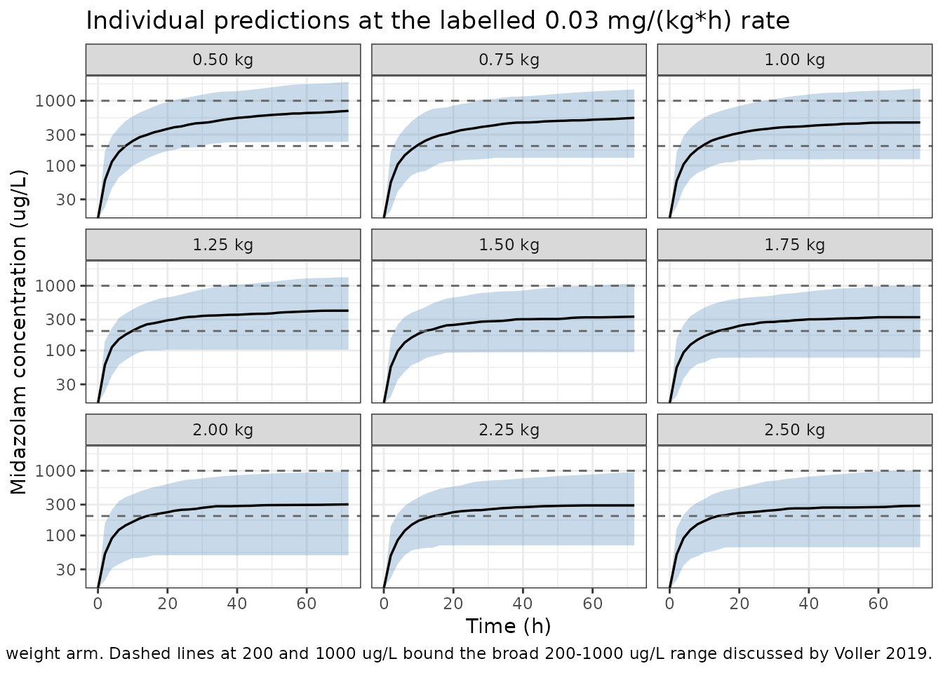
The bands are wide, which is the point the Discussion makes: with an omega of 0.919 on clearance the model places only about 65% of neonates inside even the very broad 200-1000 ug/L window under the labelled regimen.
PKNCA validation
Voller 2019 reports no non-compartmental parameters of its own, so
there is no published NCA table to compare against. What NCA can do here
is recover the model’s published structural parameters from simulated
profiles: for a one-compartment intravenous model,
CL = dose / AUCinf and Vz = CL / lambda_z
exactly, so a non-compartmental analysis of typical-value profiles must
return the Table 2 clearance and volume functions at every body weight.
That exercises the whole implementation end to end – the ODE, the
covariate functions, the centring weight, and the ug-to-L unit
convention that makes Cc come out in ug/L.
The simulated design is study 2’s: a single 0.1 mg/kg dose infused over 30 minutes. The observation grid is extended past the paper’s 24 hours to 168 hours so that the extrapolated tail of AUCinf is negligible (the slowest arm, 0.5 kg, has a half-life near 17 hours, so 168 hours is about ten half-lives). Random effects are zeroed, so both sides of the comparison are the same deterministic quantity and a tight tolerance is the correct choice.
nca_times <- c(0, 0.25, 0.5, 0.75, 1, 1.5, 2, 3, 4, 6, 8, 10, 12, 16, 20,
               24, 30, 36, 48, 60, 72, 96, 120, 144, 168)

ev_nca <- make_infusion_events(WEIGHTS, n = 1L, rate_mgkgh = 0.2,
                               dur_h = 0.5, obs_times = nca_times)

sim_nca_raw <- rxode2::rxSolve(mod_typ, events = ev_nca,
                               keep = c("WT", "treatment"))
#> ℹ omega/sigma items treated as zero: 'etalcl', 'etalvc'
#> Warning: multi-subject simulation without without 'omega'
The 0.1 mg/kg dose over 30 minutes is supplied as a rate of 0.2 mg/(kg*h) for 0.5 h, which is the same total amount.
# Filter on !is.na(Cc) only. Adding `time > 0` or `Cc > 0` would drop the
# time-zero record that PKNCA needs to anchor AUC0-inf.
sim_nca <- as.data.frame(sim_nca_raw) |>
  filter(!is.na(Cc)) |>
  select(id, time, Cc, treatment)

sim_nca <- bind_rows(
  sim_nca,
  sim_nca |> distinct(id, treatment) |> mutate(time = 0, Cc = 0)
) |>
  distinct(id, treatment, time, .keep_all = TRUE) |>
  arrange(id, treatment, time)

dose_df <- ev_nca |>
  filter(evid == 1) |>
  select(id, time, amt, treatment)

conc_obj <- PKNCA::PKNCAconc(sim_nca, Cc ~ time | treatment + id,
                             concu = "ug/L", timeu = "h")
dose_obj <- PKNCA::PKNCAdose(dose_df, amt ~ time | treatment + id,
                             doseu = "ug", route = "intravascular",
                             duration = 0.5)

intervals <- data.frame(
  start = 0, end = Inf,
  cmax = TRUE, tmax = TRUE, aucinf.obs = TRUE, half.life = TRUE,
  cl.obs = TRUE, vz.obs = TRUE
)

nca_res <- PKNCA::pk.nca(PKNCA::PKNCAdata(conc_obj, dose_obj,
                                          intervals = intervals))
published_nca <- tibble(WT = WEIGHTS) |>
  transmute(
    treatment = sprintf("%.2f kg", WT),
    cl.obs = cl_typ(WT),
    vz.obs = v_typ(WT),
    half.life = log(2) * v_typ(WT) / cl_typ(WT),
    aucinf.obs = 0.1 * WT * 1000 / cl_typ(WT)
  )

cmp <- nlmixr2lib::ncaComparisonTable(
  simulated = nca_res,
  reference = published_nca,
  by = "treatment",
  params = c("cl.obs", "vz.obs", "half.life", "aucinf.obs"),
  units = c(cl.obs = "L/h", vz.obs = "L", half.life = "h",
            aucinf.obs = "ug*h/L"),
  tolerance_pct = 5
)

knitr::kable(
  cmp,
  caption = paste(
    "Non-compartmental parameters recovered from typical-value profiles after",
    "a single 0.1 mg/kg intravenous dose over 30 min, against the Voller 2019",
    "Table 2 clearance and volume functions evaluated at the same weight.",
    "* differs from the reference by more than 5%."
  )
)| NCA parameter | treatment | Reference | Simulated | % diff |
|---|---|---|---|---|
| AUC0-∞ (obs) (ug*h/L) | 0.50 kg | 2650 | 2650 | -0.0% |
| AUC0-∞ (obs) (ug*h/L) | 0.75 kg | 2000 | 2000 | -0.0% |
| AUC0-∞ (obs) (ug*h/L) | 1.00 kg | 1640 | 1640 | -0.0% |
| AUC0-∞ (obs) (ug*h/L) | 1.25 kg | 1410 | 1410 | -0.0% |
| AUC0-∞ (obs) (ug*h/L) | 1.50 kg | 1240 | 1240 | -0.0% |
| AUC0-∞ (obs) (ug*h/L) | 1.75 kg | 1120 | 1120 | -0.0% |
| AUC0-∞ (obs) (ug*h/L) | 2.00 kg | 1020 | 1020 | -0.0% |
| AUC0-∞ (obs) (ug*h/L) | 2.25 kg | 939 | 939 | -0.0% |
| AUC0-∞ (obs) (ug*h/L) | 2.50 kg | 873 | 873 | -0.0% |
| t½ (h) | 0.50 kg | 16.9 | 16.9 | -0.0% |
| t½ (h) | 0.75 kg | 12.8 | 12.8 | -0.0% |
| t½ (h) | 1.00 kg | 10.5 | 10.5 | -0.0% |
| t½ (h) | 1.25 kg | 8.98 | 8.98 | -0.0% |
| t½ (h) | 1.50 kg | 7.92 | 7.92 | -0.0% |
| t½ (h) | 1.75 kg | 7.12 | 7.12 | +0.0% |
| t½ (h) | 2.00 kg | 6.49 | 6.49 | -0.0% |
| t½ (h) | 2.25 kg | 5.99 | 5.99 | -0.0% |
| t½ (h) | 2.50 kg | 5.57 | 5.57 | +0.0% |
| CL/F (L/h) | 0.50 kg | 0.0189 | 0.0189 | +0.0% |
| CL/F (L/h) | 0.75 kg | 0.0374 | 0.0374 | +0.0% |
| CL/F (L/h) | 1.00 kg | 0.0609 | 0.0609 | +0.0% |
| CL/F (L/h) | 1.25 kg | 0.0887 | 0.0887 | +0.0% |
| CL/F (L/h) | 1.50 kg | 0.121 | 0.121 | +0.0% |
| CL/F (L/h) | 1.75 kg | 0.157 | 0.157 | +0.0% |
| CL/F (L/h) | 2.00 kg | 0.196 | 0.196 | +0.0% |
| CL/F (L/h) | 2.25 kg | 0.24 | 0.24 | +0.0% |
| CL/F (L/h) | 2.50 kg | 0.286 | 0.286 | +0.0% |
| Vz/F (L) | 0.50 kg | 0.46 | 0.46 | +0.0% |
| Vz/F (L) | 0.75 kg | 0.69 | 0.69 | +0.0% |
| Vz/F (L) | 1.00 kg | 0.92 | 0.92 | +0.0% |
| Vz/F (L) | 1.25 kg | 1.15 | 1.15 | +0.0% |
| Vz/F (L) | 1.50 kg | 1.38 | 1.38 | +0.0% |
| Vz/F (L) | 1.75 kg | 1.61 | 1.61 | +0.0% |
| Vz/F (L) | 2.00 kg | 1.84 | 1.84 | +0.0% |
| Vz/F (L) | 2.25 kg | 2.07 | 2.07 | +0.0% |
| Vz/F (L) | 2.50 kg | 2.3 | 2.3 | +0.0% |
nca_wide <- as.data.frame(nca_res$result) |>
  filter(PPTESTCD %in% c("cl.obs", "vz.obs", "half.life")) |>
  select(treatment, PPTESTCD, PPORRES) |>
  pivot_wider(names_from = PPTESTCD, values_from = PPORRES) |>
  inner_join(
    published_nca |> rename(cl_ref = cl.obs, vz_ref = vz.obs,
                            hl_ref = half.life),
    by = "treatment"
  ) |>
  mutate(
    cl_pct = 100 * (cl.obs - cl_ref) / cl_ref,
    vz_pct = 100 * (vz.obs - vz_ref) / vz_ref,
    hl_pct = 100 * (half.life - hl_ref) / hl_ref
  )

nca_wide |>
  select(treatment, cl_pct, vz_pct, hl_pct) |>
  rename(
    "Body weight" = treatment,
    "CL recovery error (%)" = cl_pct,
    "Vz recovery error (%)" = vz_pct,
    "Half-life recovery error (%)" = hl_pct
  ) |>
  knitr::kable(
    digits = 2,
    caption = paste(
      "Error in recovering the published CL(WT) and V(WT) functions by",
      "non-compartmental analysis of the simulated profiles."
    )
)| Body weight | CL recovery error (%) | Vz recovery error (%) | Half-life recovery error (%) |
|---|---|---|---|
| 0.50 kg | 0.00 | 0.00 | 0 |
| 0.75 kg | 0.00 | 0.00 | 0 |
| 1.00 kg | 0.00 | 0.00 | 0 |
| 1.25 kg | 0.00 | 0.00 | 0 |
| 1.50 kg | 0.00 | 0.00 | 0 |
| 1.75 kg | 0.00 | 0.00 | 0 |
| 2.00 kg | 0.01 | 0.01 | 0 |
| 2.25 kg | 0.01 | 0.01 | 0 |
| 2.50 kg | 0.01 | 0.01 | 0 |
# Both sides are the same deterministic quantity: random effects are zeroed and
# no residual error is added, so the only difference is trapezoidal integration
# error on the AUC and the finite observation grid used for lambda_z. That is a
# pure numerical-error comparison, so a tight bound is correct here. 2% leaves
# room for the trapezoid on the infusion-phase rise while failing on any
# structural, covariate or unit error, which would move these by tens of
# percent or more.
stopifnot(
  max(abs(nca_wide$cl_pct)) < 2,
  max(abs(nca_wide$vz_pct)) < 2,
  max(abs(nca_wide$hl_pct)) < 2
)
Clearance, volume and half-life are recovered across the full 0.5-2.5 kg range, which confirms that the packaged model reproduces the published covariate functions, not merely the value at the centring weight.
Assumptions and deviations
Scale of the Table 2 random effects. Table 2 reports the interindividual variability on clearance and volume as bare percentages (91.9% and 67.2%) without naming the convention. The model file reads them as
omegadirectly, soomega^2(CL) = 0.844561andomega^2(V) = 0.451584. This is not an assumption made for convenience: it is established quantitatively in the “interindividual-variability scale” section above against the eight tail probabilities the paper reports from its own simulation, which the alternative exact-log-normal-CV reading misses by up to a factor of two. The choice is also internally consistent with the residual-error rows of the same table, which are plainly standard deviations.No correlation between the random effects. Table 2 reports the two interindividual variabilities as separate rows with no off-diagonal term and no
$OMEGA BLOCKis described, so they are entered as independent diagonal elements. A correlation, if the authors estimated one, is not reported.Covariate-centring weight. Table 1 gives the combined-cohort median actual body weight as 1.1 kg, while the Table 2 footnote states the centring value as 1.12 kg. The model uses 1.12 kg, which is the value the footnote attaches to the parameter definitions, and which reproduces the paper’s own derived concentrations exactly. The Abstract’s restatement of the estimates as being “for a neonate weighing 1.1 kg” is the Table 1 rounding of the same number.
Volume exponent encoded as
fixed(1). The Results section describes estimating a power exponent on volume, finding it “close to 1”, then testing and carrying forward the linear form. The linear form is therefore a modelling decision rather than an estimate, ande_wt_vc <- fixed(1)preserves that. The value of the estimated exponent that preceded the decision is not reported.Intravenous administration only. Both contributing studies gave midazolam intravenously, so the model has no absorption compartment and no bioavailability term. It must not be used for oral, buccal, intranasal or intramuscular midazolam without an absorption model fitted for that route.
Body weight is time-varying in the source data. The Methods describe recording actual body weight at each day in the intensive care unit and interpolating linearly between measurements, so
WTis a time-varying covariate in the estimation data set. The simulations here hold weight fixed within each arm, which is the design the paper itself used for its dosing evaluation (nine hypothetical neonates of fixed weight). Users simulating real growth trajectories should supply a time-varyingWTcolumn.Extrapolation beyond the fitted range. The pooled cohort spans gestational age 24.0-33.6 weeks and actual body weight 0.6-4.3 kg. The Discussion states explicitly that “the proposed dosing regimen could not be evaluated beyond a gestational age of 34 weeks because the population did not include individuals above that gestational age”. The 1.69 clearance exponent is far steeper than allometric and is a description of CYP3A maturation over the preterm weight range, not a size relationship; extrapolating it to term neonates, infants or children will overstate clearance badly. A 10 kg child would be assigned a clearance of about 3.5 L/h against a published value near 0.4 L/h for a one-year-old.
Observation-grid extension in the PKNCA section. Study 2 sampled to 24 hours; the NCA validation here extends the simulated grid to 168 hours so that the extrapolated tail of AUCinf is negligible and clearance can be recovered exactly. This is a property of the validation design, not of the model.
Errata
No erratum, corrigendum or author correction to Voller 2019 was found on the Wiley article landing page or in PubMed at the time of extraction.
The article’s Supporting Information (Supplemental Table S1, the
covariate analysis detail; Supplemental Figure S1, eta-versus-covariate
plots; Supplemental Figure S2, the normalized prediction distribution
error) was not obtained. None of it carries parameter values: every
final estimate, its relative standard error, its eta shrinkage and its
bootstrap confidence interval is printed in Table 2 of the main article,
and Supplemental Table S1 documents covariate steps that were screened
and rejected rather than any retained effect. The screened-and-rejected
covariates are recorded in the model file’s
covariatesDataExcluded list from the Methods and Table 1 of
the main article.
No parameter in this model came from anywhere other than the main article’s Table 2, its Results text, and the Table 2 footnote.