Matuzumab (Kuester 2008)
Source:vignettes/articles/Kuester_2008_matuzumab.Rmd
Kuester_2008_matuzumab.RmdModel and source
- Citation: Kuester K, Kovar A, Lupfert C, Brockhaus B, Kloft C. Population pharmacokinetic data analysis of three phase I studies of matuzumab, a humanised anti-EGFR monoclonal antibody in clinical cancer development. Br J Cancer. 2008;98(5):900-906. doi:10.1038/sj.bjc.6604265
- Description: Two-compartment population PK model for matuzumab (humanised anti-EGFR IgG1 monoclonal antibody) in adults with advanced carcinoma (Kuester 2008), with parallel first-order linear and Michaelis-Menten elimination from the central compartment; body weight on linear CL and central volume.
- Article: Br J Cancer. 2008;98(5):900-906
Population
Kuester 2008 pooled data from three phase I, open-label, multicentre studies of intravenous matuzumab (humanised anti-EGFR IgG1 mAb) in adults with advanced, non-resectable and/or metastatic carcinoma (Kuester 2008 Methods, p901). The final dataset contained 1256 serum concentration-time measurements from 90 patients (53 male / 37 female) ranging from 0.258 to 1157 ug/mL across 11 dosing regimens.
Baseline demographics (Kuester 2008 Table 2, p902): median age 60 years (range 29-82), median body weight 71 kg (range 44-125), median height 169 cm (range 143-198), median BSA 1.82 m^2 (range 1.34-2.59), median BMI 24.9 kg/m^2 (range 15.9-37.0), median creatinine clearance 91 mL/min (range 41-480), median alkaline phosphatase 171 U/L, median lactate dehydrogenase 426 U/L. Tumour entities: advanced pancreatic cancer (study 1, n = 17) or various advanced carcinoma predominantly colorectal (study 2 n = 51; study 3 n = 22). Concomitant chemotherapy (fixed-dose gemcitabine 1000 mg/m^2) was administered to all 17 study-1 patients only.
Matuzumab was given as 1-hour IV infusions of 400-2000 mg in 11 different regimens spanning q1w, q2w, and q3w schedules; some patients were treated for ~1 year (Kuester 2008 Methods, p901; Table 1).
The same information is available programmatically via
readModelDb("Kuester_2008_matuzumab")$population.
Source trace
Every structural parameter, covariate effect, IIV element, and residual-error term below is taken from Kuester 2008 Table 3 (final-model column, p902). The reference covariate value is WT = 71 kg, the pooled cohort median (Table 2). All times are in hours; clearances in L/h; volumes in L; Vmax in mg/h; Km and concentrations in ug/mL (= mg/L).
| Equation / parameter | Value | Source location |
|---|---|---|
lcl (CLL) |
log(14.5/1000) L/h |
Table 3 CLL = 14.5 mL/h (RSE 4.1%) |
lvc (V1) |
log(3.72) L |
Table 3 V1 = 3.72 L (RSE 3.0%) |
lq (Q) |
log(38.3/1000) L/h |
Table 3 Q = 38.3 mL/h (RSE 7.6%) |
lvp (V2) |
log(1.84) L |
Table 3 V2 = 1.84 L (RSE 9.0%) |
lvmax (Vmax) |
log(0.456) mg/h |
Table 3 Vmax = 0.456 mg/h (RSE 13.7%) |
lkm (Km) |
log(4.0) ug/mL |
Table 3 Km = 4.0 mg/L = 4.0 ug/mL (RSE 29.8%) |
e_wt_vc (linear coef on V1) |
0.0044 per kg |
Table 3 V1_WT = +0.44% per kg (RSE 35.2%) |
e_wt_cl (linear coef on CLL) |
0.0087 per kg |
Table 3 CLL_WT = +0.87% per kg (RSE 28.2%) |
var(etalcl) |
log(1 + 0.240^2) = 0.05598 |
Table 3 IIV CLL = 24.0% CV (RSE 20.5%) |
var(etalvc) |
log(1 + 0.219^2) = 0.04685 |
Table 3 IIV V1 = 21.9% CV (RSE 20.3%) |
var(etalvp) |
log(1 + 0.616^2) = 0.32149 |
Table 3 IIV V2 = 61.6% CV (RSE 27.6%) |
var(etalvmax) |
log(1 + 0.538^2) = 0.25416 |
Table 3 IIV Vmax = 53.8% CV (RSE 38.1%) |
cor(etalvc, etalvp) |
0.777 |
Table 3 Correlation V1_V2 (RSE 29.8%) |
cor(etalvc, etalvmax) |
0.875 |
Table 3 Correlation V1_Vmax (RSE 28.4%) |
cor(etalvp, etalvmax) |
0.875 |
Table 3 Correlation V2_Vmax (RSE 31.6%) |
propSd |
0.134 |
Table 3 Residual proportional = 13.4% CV (RSE 1.5%) |
addSd |
fixed(0.312) ug/mL |
Table 3 Residual additive = 0.312 mg/L (fixed) |
| Structure (2-cmt + parallel linear + MM elimination from central) | n/a | Methods p901; Figure 2 p902 |
Parameterization notes
-
Two-compartment IV with parallel linear and Michaelis-Menten
elimination from the central compartment. Kuester 2008 fits a
2-compartment model with first-order linear clearance
CLL(mL/h) and saturable Michaelis-Menten elimination withVmax(mg/h) andKm(mg/L) acting on the central compartment (Figure 2, p902). “Implementation of CLNL from the peripheral compartment only or from both compartments did not result in an improvement of the model” (Results, p903), so the nonlinear pathway is fromcentralonly. Total clearance at low concentrations (Cc << Km) is the sum CLL + Vmax/Km = 14.5 + 0.456/4.0 * 1000 = 14.5 + 114.0 = 128.5 mL/h (final-model values reported in the Results, p904 give 14.5 + 114.0 = 128.5 mL/h vs the paper-stated 118.8 mL/h computed from the base-model values 14.6 + 104.2; the small difference reflects the base-vs-final parameter update). Dose enterscentraldirectly via the 1-hour IV infusion; there is no depot compartment. -
Linear additive-offset covariate form (not
power-of-ratio). Kuester 2008 uses the linear additive-offset
form
V1 = V1_typ * (1 + V1_WT * (WT - 71))and analogous for CLL (Table 3 footnotes c and d, p902), rather than the more common power-of-ratio(WT / 71)^exponent. With V1_WT = 0.0044 and CLL_WT = 0.0087, a 10 kg increase from the median raises V1 by 4.4% and CLL by 8.7%. The paper reports a -19% to +25% range across the 5th to 95th WT percentile. -
CV% to log-normal variance and correlated IIV
block. Kuester 2008 Table 3 reports IIV as CV% on the
linear-parameter scale. Convert via
omega^2 = log(1 + CV^2). The off-diagonal covariances followcov_ij = r_ij * sqrt(omega_i^2 * omega_j^2)using the three reported correlation coefficients V1-V2, V1-Vmax, and V2-Vmax. IIV on CLL is independent (no correlations involving CLL were reported). -
Residual additive term held fixed. The additive
component (0.312 mg/L = 0.312 ug/mL) was fixed by the authors “due to
model stability (the value was chosen from prior plausible successfully
run models)” (Results, p904). The model file wraps it in
fixed()so the provenance is visible in?modellib.
Errata
No errata or corrigenda located for this paper (PubMed search 2026-06-04; BJC corrections feed search).
Virtual cohort
The simulations below use a virtual cohort whose weight distribution approximates the Kuester 2008 Table 2 demographics. No subject-level observed data were released with the paper.
set.seed(20260604)

# 200 subjects per dose arm gives stable 5/50/95 percentile bands for the
# Figure 1 reproduction and the PKNCA distribution summaries.
n_subj <- 200

clamp <- function(x, lo, hi) pmin(pmax(x, lo), hi)

cohort <- tibble::tibble(
  id = seq_len(n_subj),
  # Weight: median 71 kg, observed range 44-125 (Kuester 2008 Table 2).
  # Approximate the distribution with a clamped log-normal whose 5-95th
  # percentiles span the bulk of the published range.
  WT = clamp(rlnorm(n_subj, meanlog = log(70), sdlog = 0.20), 44, 125)
)
Four weekly (q1w) dosing regimens are simulated in parallel: 400, 800, 1200, and 1600 mg by 1-hour IV infusion for four cycles. This reproduces the sampling structure of Kuester 2008 Figure 1, which compares concentration-time profiles after the first infusion (left panel) and after the fourth infusion (right panel).
tau     <- 168   # weekly dosing interval (hours)
inf_dur <- 1     # 1-hour IV infusion duration
n_doses <- 4
dose_hours <- seq(0, tau * (n_doses - 1), by = tau)

dose_levels <- c(400, 800, 1200, 1600)

build_events <- function(cohort, dose_mg, treatment, id_offset = 0L) {
  cohort <- cohort |> dplyr::mutate(id = id + id_offset)
  ev_dose <- cohort |>
    tidyr::crossing(time = dose_hours) |>
    dplyr::mutate(amt = dose_mg,
                  cmt = "central",
                  evid = 1L,
                  dur  = inf_dur,
                  treatment = treatment)
  # Observation grid: dense after the first infusion (to capture distribution
  # phase) and after the fourth infusion (~Figure 1 right panel), with a
  # coarser grid in between.
  obs_hours <- sort(unique(c(
    0, 0.5, 1, 1.25, 1.5, 2, 3, 5, 8, 12, 24, 48, 72, 96, 120, 144,
    seq(168, tau * (n_doses - 1) - 1, by = 24),
    seq(tau * (n_doses - 1), tau * n_doses, by = 2),
    dose_hours + inf_dur,
    dose_hours + 24, dose_hours + 72
  )))
  ev_obs <- cohort |>
    tidyr::crossing(time = obs_hours) |>
    dplyr::mutate(amt = 0, cmt = NA_character_, evid = 0L,
                  dur = NA_real_, treatment = treatment)
  dplyr::bind_rows(ev_dose, ev_obs) |>
    dplyr::arrange(id, time, dplyr::desc(evid)) |>
    dplyr::select(id, time, amt, cmt, evid, dur, treatment, WT)
}

events <- dplyr::bind_rows(
  lapply(seq_along(dose_levels), function(i) {
    build_events(cohort, dose_levels[i],
                 paste0(dose_levels[i], " mg q1w"),
                 id_offset = (i - 1L) * n_subj)
  })
)
stopifnot(!anyDuplicated(unique(events[, c("id", "time", "evid")])))
Simulation
mod <- rxode2::rxode2(readModelDb("Kuester_2008_matuzumab"))
#> ℹ parameter labels from comments will be replaced by 'label()'
conc_unit <- mod$units[["concentration"]]
keep_cols <- c("WT", "treatment")

sim <- lapply(split(events, events$treatment), function(ev) {
  out <- rxode2::rxSolve(mod, events = ev, keep = keep_cols)
  as.data.frame(out)
}) |> dplyr::bind_rows()
Replicate published figures
Figure 1 – concentration-time profiles after first and fourth infusion
Kuester 2008 Figure 1 (p903) shows semilogarithmic geometric-mean +/- SD observed concentration-time profiles of the four weekly dose regimens (400, 800, 1200, 1600 mg q1w) after the first infusion (left panel) and after the fourth infusion (right panel). The blocks below replicate both panels using the simulated geometric-mean +/- geometric-SD profiles.
first_inf <- sim |>
  dplyr::filter(!is.na(Cc), Cc > 0, time >= 0, time <= tau) |>
  dplyr::group_by(treatment, time) |>
  dplyr::summarise(
    log_mean = mean(log(Cc)),
    log_sd   = sd(log(Cc)),
    .groups  = "drop"
  ) |>
  dplyr::mutate(
    geomean = exp(log_mean),
    gsdlow  = exp(log_mean - log_sd),
    gsdhigh = exp(log_mean + log_sd)
  )

ggplot(first_inf, aes(time, geomean, colour = treatment, fill = treatment)) +
  geom_ribbon(aes(ymin = pmax(gsdlow, 0.1), ymax = gsdhigh),
              alpha = 0.18, colour = NA) +
  geom_line(linewidth = 0.8) +
  scale_y_log10() +
  labs(
    x = "Time after first infusion (h)",
    y = paste0("Matuzumab Cc (", conc_unit, ", log scale)"),
    title = "Replicates Kuester 2008 Figure 1, left panel",
    caption = "Geometric mean (line) and geometric-SD interval (shaded) after the first weekly infusion."
  ) +
  theme_minimal()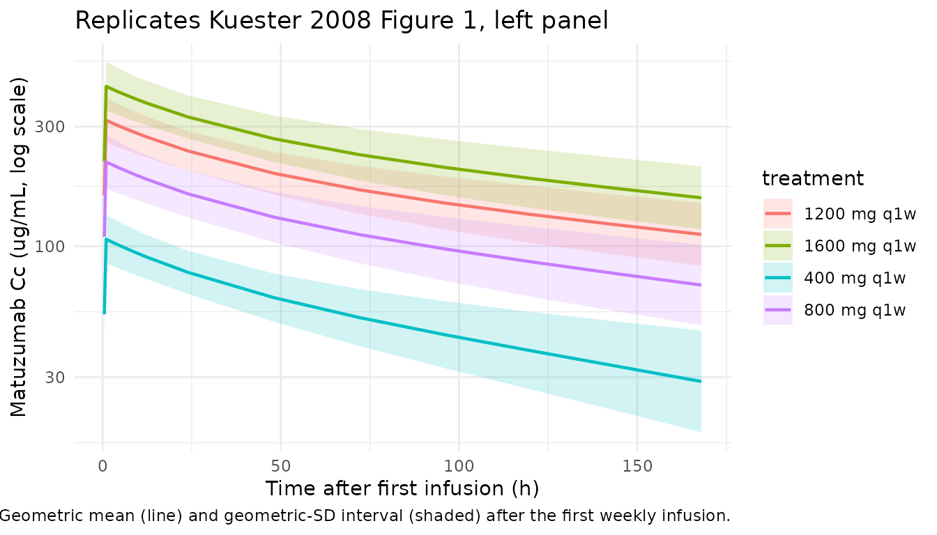
ss_start <- tau * (n_doses - 1)

fourth_inf <- sim |>
  dplyr::filter(!is.na(Cc), Cc > 0, time >= ss_start, time <= ss_start + tau) |>
  dplyr::mutate(time_rel = time - ss_start) |>
  dplyr::group_by(treatment, time_rel) |>
  dplyr::summarise(
    log_mean = mean(log(Cc)),
    log_sd   = sd(log(Cc)),
    .groups  = "drop"
  ) |>
  dplyr::mutate(
    geomean = exp(log_mean),
    gsdlow  = exp(log_mean - log_sd),
    gsdhigh = exp(log_mean + log_sd)
  )

ggplot(fourth_inf, aes(time_rel, geomean, colour = treatment, fill = treatment)) +
  geom_ribbon(aes(ymin = pmax(gsdlow, 0.1), ymax = gsdhigh),
              alpha = 0.18, colour = NA) +
  geom_line(linewidth = 0.8) +
  scale_y_log10() +
  labs(
    x = "Time after fourth infusion (h)",
    y = paste0("Matuzumab Cc (", conc_unit, ", log scale)"),
    title = "Replicates Kuester 2008 Figure 1, right panel",
    caption = "Geometric mean (line) and geometric-SD interval (shaded) after the fourth weekly infusion."
  ) +
  theme_minimal()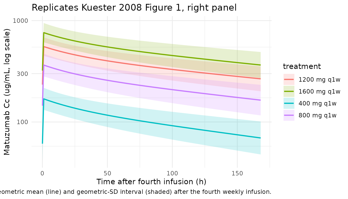
Figure 3 – concentration dependence of total clearance and half-life
Kuester 2008 Figure 3 (p903) shows total clearance and apparent half-life as a function of mAb concentration. The block below uses the typical-value parameter set (no IIV) to reproduce the same shape: clearance drops with increasing concentration as the saturable pathway is filled up, and the apparent first-order rate from the central compartment lengthens.
# Final-model typical values from Table 3 (with mass-balance units chosen
# so unit conversions stay explicit):
CLL_mlh   <- 14.5             # linear CL in mL/h
Vmax_ugh  <- 0.456 * 1000     # Vmax in ug/h (0.456 mg/h = 456 ug/h)
Km_ugml   <- 4.0              # Km in ug/mL
V1_L      <- 3.72             # central volume in L

C_grid <- exp(seq(log(0.1), log(2000), length.out = 200))

# Concentration-dependent nonlinear clearance:
#   CL_nl(C) = Vmax / (Km + C)
# Vmax [ug/h] / (Km + C) [ug/mL] = mL/h. Total CL is the sum of linear and
# nonlinear arms; apparent first-order rate constant from the central
# compartment is CL_total / V1.
CL_nl_mlh    <- Vmax_ugh / (Km_ugml + C_grid)               # mL/h
CL_total_mlh <- CLL_mlh + CL_nl_mlh                         # mL/h
k_app_per_h  <- (CL_total_mlh / 1000) / V1_L                # 1/h
half_life_d  <- log(2) / k_app_per_h / 24                   # days

clearance_df <- tibble::tibble(
  C        = C_grid,
  CL_total = CL_total_mlh,
  CL_lin   = CLL_mlh,
  CL_nl    = CL_nl_mlh,
  t_half_d = half_life_d
)

p_cl <- ggplot(clearance_df, aes(C)) +
  geom_line(aes(y = CL_total, colour = "Total"), linewidth = 0.8) +
  geom_line(aes(y = CL_lin,   colour = "Linear"), linewidth = 0.6, linetype = "dashed") +
  geom_line(aes(y = CL_nl,    colour = "Nonlinear"), linewidth = 0.6, linetype = "dotted") +
  scale_x_log10() +
  labs(x = "Matuzumab Cc (ug/mL, log scale)",
       y = "Clearance (mL/h)",
       colour = "Component",
       title = "Replicates Kuester 2008 Figure 3, left panel") +
  theme_minimal()

p_th <- ggplot(clearance_df, aes(C, t_half_d)) +
  geom_line(linewidth = 0.8) +
  scale_x_log10() +
  labs(x = "Matuzumab Cc (ug/mL, log scale)",
       y = "Apparent half-life (days)",
       title = "Replicates Kuester 2008 Figure 3, right panel") +
  theme_minimal()

p_cl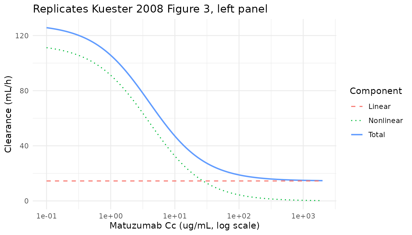
p_th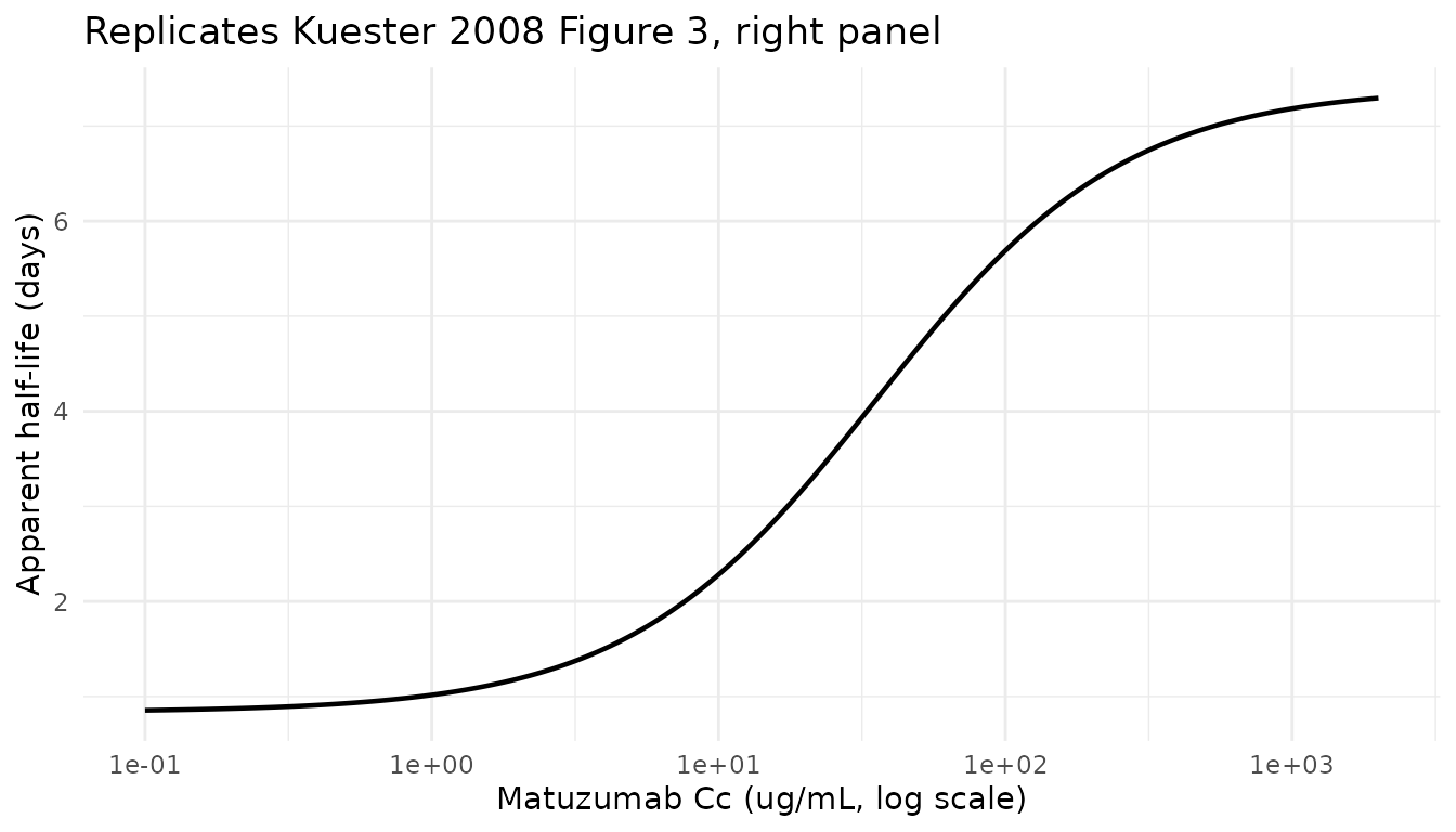
Reading off the plot at the two anchor concentrations reported in the text:
anchor_df <- tibble::tibble(
  C = c(20, 1000),
  t_half_d = log(2) /
    (((CLL_mlh + Vmax_ugh / (Km_ugml + C)) / 1000) / V1_L) / 24
)
anchor_df |>
  dplyr::rename(
    "Cc (ug/mL)"           = C,
    "Apparent t1/2 (days)" = t_half_d
  ) |>
  knitr::kable(digits = 2,
  caption = paste("Apparent first-order half-life from the central compartment.",
                  "Kuester 2008 reports 4.4 d at 20 ug/mL and 10.5 d at 1000 ug/mL",
                  "(Results, p904; Figure 3 right panel). The two-compartment terminal",
                  "half-life is longer than the apparent first-order value computed here",
"because it includes contributions from peripheral redistribution."))| Cc (ug/mL) | Apparent t1/2 (days) |
|---|---|
| 20 | 3.21 |
| 1000 | 7.18 |
PKNCA validation
The block below runs non-compartmental analysis on the simulated concentration profiles after the first weekly infusion to give Cmax, Tmax, and AUC0-tau (tau = 168 h) per simulated subject and dose group. Kuester 2008 does not publish an NCA table, so the comparison below is internal: AUC0-tau is expected to scale approximately with dose (slightly super-proportionally because the saturable pathway clears less of the larger doses), and Cmax should occur near the end of the 1-hour infusion.
nca_conc <- sim |>
  dplyr::filter(time >= 0, time < tau, !is.na(Cc)) |>
  dplyr::select(id, time, Cc, treatment)

nca_dose <- events |>
  dplyr::filter(evid == 1, time == 0) |>
  dplyr::select(id, time, amt, treatment)

conc_obj <- PKNCA::PKNCAconc(nca_conc, Cc ~ time | treatment + id)
dose_obj <- PKNCA::PKNCAdose(nca_dose, amt ~ time | treatment + id)

intervals <- data.frame(
  start      = 0,
  end        = tau,
  cmax       = TRUE,
  tmax       = TRUE,
  auclast    = TRUE,
  half.life  = TRUE
)

nca_res <- PKNCA::pk.nca(PKNCA::PKNCAdata(conc_obj, dose_obj, intervals = intervals))
summary(nca_res)
#>  start end   treatment   N      auclast       cmax              tmax  half.life
#>      0 168 1200 mg q1w 200 26300 [21.4] 318 [21.0] 1.00 [1.00, 1.00] 176 [41.3]
#>      0 168 1600 mg q1w 200 36300 [22.9] 434 [22.8] 1.00 [1.00, 1.00] 183 [44.0]
#>      0 168  400 mg q1w 200  8230 [25.1] 107 [22.4] 1.00 [1.00, 1.00] 128 [34.1]
#>      0 168  800 mg q1w 200 17500 [25.8] 217 [25.0] 1.00 [1.00, 1.00] 158 [42.0]
#>
#> Caption: auclast, cmax: geometric mean and geometric coefficient of variation; tmax: median and range; half.life: arithmetic mean and standard deviation; N: number of subjects
Dose-proportionality summary
nca_long <- as.data.frame(nca_res$result)

per_subj <- nca_long |>
  dplyr::filter(PPTESTCD %in% c("cmax", "tmax", "auclast", "half.life")) |>
  tidyr::pivot_wider(id_cols = c(treatment, id),
                     names_from = PPTESTCD, values_from = PPORRES)

dose_summary <- per_subj |>
  dplyr::group_by(treatment) |>
  dplyr::summarise(
    Cmax_mean      = mean(cmax, na.rm = TRUE),
    Cmax_sd        = sd(cmax,   na.rm = TRUE),
    Tmax_mean      = mean(tmax, na.rm = TRUE),
    AUC0_tau_mean  = mean(auclast, na.rm = TRUE),
    AUC0_tau_sd    = sd(auclast,   na.rm = TRUE),
    HalfLife_mean  = mean(half.life, na.rm = TRUE),
    .groups = "drop"
  )

knitr::kable(dose_summary, digits = 2,
  caption = paste("Simulated single-dose NCA parameters by dose group",
                  "(0-168 h after the first weekly infusion).",
"Cmax (ug/mL), AUC0-tau (ug/mL * h), Tmax / half-life in hours."))| treatment | Cmax_mean | Cmax_sd | Tmax_mean | AUC0_tau_mean | AUC0_tau_sd | HalfLife_mean |
|---|---|---|---|---|---|---|
| 1200 mg q1w | 324.91 | 69.78 | 1 | 26923.94 | 5882.23 | 176.47 |
| 1600 mg q1w | 445.42 | 101.33 | 1 | 37211.96 | 8628.76 | 183.34 |
| 400 mg q1w | 109.19 | 23.96 | 1 | 8478.38 | 2066.48 | 128.08 |
| 800 mg q1w | 223.49 | 54.24 | 1 | 18060.76 | 4498.11 | 158.48 |
Assumptions and deviations
- Virtual-cohort covariate distributions. Body weight is drawn from a clamped log-normal with the Kuester 2008 Table 2 median 71 kg and an approximate sdlog of 0.20 to span most of the observed 44-125 kg range. No other covariates were retained in the final model.
- No subject-level observed data. Kuester 2008 does not release subject-level concentrations; the validation reproduces the geometric-mean +/- SD bands of Figure 1 and the clearance / half-life curves of Figure 3 rather than overlaying observed points.
- Inter-occasion variability not encoded structurally. Kuester 2008 reports IOV on CLL (22.8% CV, Table 3) with every infusion treated as one occasion. There is no standardized OCC indicator in the nlmixr2lib event-data schema, so IOV is omitted in the model file. Downstream users who want to simulate IOV can add an OCC indicator column to the event dataset and a per-occasion eta in rxode2.
- Apparent half-life vs terminal half-life. The Figure 3 reproduction above uses the apparent first-order rate from the central compartment (linear + Michaelis-Menten contributions divided by V1). This matches the shape and order of magnitude of the paper’s Figure 3 right panel (4.4 d at 20 ug/mL, 10.5 d at 1000 ug/mL). The true 2-compartment terminal half-life is longer than this apparent value because it includes the peripheral-redistribution contribution.
-
Dosing assumption. Doses are administered as 1-hour
IV infusions with
dur = 1, matching Kuester 2008 Methods (p901). The first sample after each infusion is taken from the simulated grid at t = 1.25 h (immediately after the end of infusion) to approximate the paper’s near-end-of-infusion peak sampling.