Metoprolol gender-based dose equivalence in adults (Eugene 2016, Med Sci) • nlmixr2lib

library(nlmixr2lib)
library(rxode2)
library(PKNCA)
library(dplyr)
library(tibble)
library(ggplot2)
rxode2::rxSetSeed(20161115)

Eugene AR. Metoprolol Dose Equivalence in Adult Men and Women Based on Gender Differences: Pharmacokinetic Modeling and Simulations. Med Sci (Basel). 2016;4(4):18. doi:10.3390/medsci4040018.

This paper asks a single clinical question: what oral metoprolol dose in women gives the same total exposure as 100 mg in men? Its answer – 50 mg – rests on a one-compartment PK model fit to digitized mean concentration-time curves from Luzier 1999, and the paper contributes two distinct parameter sets:

Paper table	What it is	Model file
Table 1	Fit to the digitized Luzier 1999 curves; both R- and S-metoprolol, sex-stratified; typical values only	`Eugene_2016b_metoprolol_enantiomers`
Table 2	Re-fit of the paper’s own 100-subject Clinical Trial Simulation; S-metoprolol only; carries inter-individual variability	`Eugene_2016b_metoprolol`

Both are extracted. Table 1 is the model that actually generates every published Cmax / Tmax / AUC / half-life number in the paper (Results 3.2), so it carries the quantitative validation below; Table 2 is the only one of the two with random effects, so it carries the stochastic cohort simulation.

Not to be confused with Eugene_2016a_metoprolol, a different Eugene 2016 metoprolol paper (Int J Clin Pharmacol Toxicol 5(3):209-215, doi:10.19070/2167-910X-1600035), which models chronically ill elderly inpatients. The two papers share an author, a year and a drug but have different cohorts, data sources and parameter values. They are distinguished by the a (May 2016, elderly) and b (November 2016, healthy young adults) year suffixes.

mod_enant <- rxode2::rxode2(readModelDb("Eugene_2016b_metoprolol_enantiomers"))
mod_cts <- rxode2::rxode2(readModelDb("Eugene_2016b_metoprolol"))
#> ℹ parameter labels from comments will be replaced by 'label()'

Citation: Eugene AR. (2016). Metoprolol Dose Equivalence in Adult Men and Women Based on Gender Differences: Pharmacokinetic Modeling and Simulations. Med Sci (Basel) 4(4):18. doi:10.3390/medsci4040018.
Enantiomer model: Enantiomer-resolved one-compartment PK model for oral metoprolol in healthy young adults, tracking R-metoprolol and S-metoprolol in parallel with first-order absorption and an absorption lag time and with every structural parameter stratified by sex. Typical values only (no inter-individual variability was estimated). The kinetics are flip-flop: absorption is rate-limiting, so the terminal slope is set by Ka rather than by CL/V. These are the parameters that generate every published Cmax, Tmax, AUC and half-life in Eugene 2016 (Eugene 2016).
CTS model: One-compartment population PK model for oral S-metoprolol with first-order absorption and an absorption lag time in healthy young adults; every structural parameter is stratified by sex, and the kinetics are flip-flop (absorption is rate-limiting). Estimated by re-fitting the paper’s own 100-subject Clinical Trial Simulation, so this is the variant of the Eugene 2016 Med Sci model that carries inter-individual variability (Eugene 2016).

Population

pop <- mod_enant$population
tibble(Field = names(pop), Value = vapply(pop, function(x) paste(x, collapse = "; "), character(1))) |>
  knitr::kable(caption = "Population metadata for the Table 1 (enantiomer) model.")

Population metadata for the Table 1 (enantiomer) model.
Field	Value
species	human
n_subjects	20
n_studies	1
age_range	20-36 years
age_median	not reported
weight_range	men 83.9 +/- 10.7 kg, women 62.0 +/- 7.3 kg (mean +/- SD, Luzier 1999 as quoted in Eugene 2016 Discussion)
weight_median	not reported (means reported instead)
sex_female_pct	50
race_ethnicity	not reported
disease_state	Healthy volunteers
dose_range	Nine 100 mg oral doses of racemic metoprolol every 12 h (Eugene 2016 Methods 2.1, citing the Luzier 1999 protocol).
regions	United States (Luzier 1999 cohort; Eugene 2016 analysis performed at Mayo Clinic, Rochester MN)
notes	n = 20 healthy volunteers (10 men, 10 women) from Luzier 1999. Eugene 2016 did not have access to the individual-level data: the mean R-metoprolol and S-metoprolol concentration-time curves were DIGITIZED from the Luzier 1999 figures, giving four distinct profiles (enantiomer x sex), and each was fit in MONOLIX 4.3.3 (SAEM-MCMC). Because the fits are to mean curves rather than individual subjects, no inter-individual variability and no residual-error magnitude are reported for this model – see the vignette Errata. Eugene 2016 undertook the fit because the original Luzier 1999 publication did not report Ka or Tlag (Methods 2.2).

The underlying clinical data are from Luzier AB et al. (1999), a crossover study in 20 healthy volunteers (10 men, 10 women), aged 20-36 years, each given nine 100 mg doses of racemic metoprolol every 12 h. Eugene 2016 did not have the individual-level data: the published mean R- and S-metoprolol curves were digitized into four profiles (enantiomer x sex) and each was fit in MONOLIX 4.3.3. The stated reason for re-fitting is that Luzier 1999 never reported Ka or Tlag (Methods 2.2).

Men in the Luzier cohort weighed 83.9 +/- 10.7 kg and women 62.0 +/- 7.3 kg. Eugene 2016 discusses that 21 kg difference as a likely contributor to the sex difference in exposure but does not include body weight in the model – sex is carried as a stratification, not as a weight-normalised term.

Source trace

Source location for every model equation and ini() parameter.
Quantity	Source location	Model file
Structural form: 1-cmt, first-order absorption, lag time	Results 3.1 (‘a one-compartment model adequately described metoprolol pharmacokinetics’); Methods 2.2	both
R-metoprolol Tlag / Ka / V / CL, male and female	Table 1, R-Metoprolol columns	enantiomers
S-metoprolol Tlag / Ka / V / CL, male and female	Table 1, S-Metoprolol columns	enantiomers
Published Cmax / Tmax / AUC / t-half, 100 mg M and F, 50 mg F	Results 3.2	validation target
CTS Tlag / Ka / V / CL, men and women	Table 2, Value columns	CTS
IIV variances (omega^2) for Tlag / Ka / V / CL	Table 2, lower block	CTS
Proportional residual error 0.0281	Table 2, ‘Proportional error model’ row	CTS
CTS design: 50 men + 50 women, 100 mg S-metoprolol, 17 sample times	Methods 2.4; Results 3.3	CTS
Per-sex CV inputs to the CTS (S-CL 59/49%, S-V 44/34%, Ka 40%)	Methods 2.4	population notes
Sex encoding (male as reference, female as log-additive offset)	Derived from Table 1 / Table 2 column pairs	both

Part 1 – The Table 1 enantiomer model

Structural parameter recovery

The model stores each enantiomer’s male column as the reference and each female value as a log-additive offset log(female / male). That is an exact re-parameterisation, so solving the model must return Table 1 verbatim.

tbl1 <- tribble(
  ~enantiomer, ~SEXF, ~tlag, ~ka,    ~vc,   ~cl,
  "S",         0,     0.67,  0.241,  55.3,  253,
  "S",         1,     0.38,  0.161,  34.9,  101,
  "R",         0,     0.59,  0.234,  63.9,  316,
  "R",         1,     0.39,  0.165,  38.1,  120
)

probe <- function(sexf) {
  ev <- bind_rows(
    tibble(id = 1L, time = 0, amt = 100, evid = 1L, cmt = "depot_s_enant", dvid = NA_integer_),
    tibble(id = 1L, time = c(0, 1), amt = NA_real_, evid = 0L, cmt = NA_character_, dvid = 2L)
  )
  s <- rxode2::rxSolve(rxode2::zeroRe(mod_enant), ev,
    params = c(SEXF = as.numeric(sexf)), returnType = "data.frame")
  s[1, ]
}

recovered <- bind_rows(lapply(c(0, 1), function(sx) {
  p <- probe(sx)
  bind_rows(
    tibble(enantiomer = "S", SEXF = sx, tlag = p$tlag_s_enant, ka = p$ka_s_enant,
      vc = p$vc_s_enant, cl = p$cl_s_enant),
    tibble(enantiomer = "R", SEXF = sx, tlag = p$tlag_r_enant, ka = p$ka_r_enant,
      vc = p$vc_r_enant, cl = p$cl_r_enant)
  )
}))
#> Warning: No omega parameters in the model
#> No omega parameters in the model

chk1 <- tbl1 |>
  left_join(recovered, by = c("enantiomer", "SEXF"), suffix = c("_pub", "_sim"))

chk1 |>
  mutate(across(where(is.numeric), ~ signif(.x, 4))) |>
  rename("Enantiomer" = enantiomer, "SEXF" = SEXF) |>
  knitr::kable(caption = "Eugene 2016 Table 1 (published, _pub) vs values recovered from the model file (_sim).")

Eugene 2016 Table 1 (published, _pub) vs values recovered from the model file (_sim).
Enantiomer	SEXF	tlag_pub	ka_pub	vc_pub	cl_pub	tlag_sim	ka_sim	vc_sim	cl_sim
S	0	0.67	0.241	55.3	253	0.67	0.241	55.3	253
S	1	0.38	0.161	34.9	101	0.38	0.161	34.9	101
R	0	0.59	0.234	63.9	316	0.59	0.234	63.9	316
R	1	0.39	0.165	38.1	120	0.39	0.165	38.1	120


# The re-parameterisation is exact arithmetic, not a fit, so this bound is
# tight on purpose: any transcription slip moves a value far more than 1e-8.
stopifnot(
  max(abs(chk1$tlag_pub - chk1$tlag_sim)) < 1e-8,
  max(abs(chk1$ka_pub - chk1$ka_sim)) < 1e-8,
  max(abs(chk1$vc_pub - chk1$vc_sim)) < 1e-8,
  max(abs(chk1$cl_pub - chk1$cl_sim)) < 1e-8
)

These kinetics are flip-flop

This is the single most important structural feature of the model, and it is not stated anywhere in the paper’s text – it has to be derived from the tabulated numbers.

For S-metoprolol in men, kel = CL/V = 253/55.3 = 4.58 1/h, giving an elimination half-life of about 9 minutes, whereas Ka = 0.241 1/h gives an absorption half-life of 2.9 h. Absorption is roughly twenty times slower than elimination, so the observed terminal slope is the absorption rate constant, not the elimination rate constant.

tbl1 |>
  mutate(
    kel = cl / vc,
    `t-half elimination (h)` = log(2) / kel,
    `t-half absorption (h)` = log(2) / ka,
    `published t-half (h)` = c(2.9, 4.3, NA, NA)
  ) |>
  select(enantiomer, SEXF, `t-half elimination (h)`, `t-half absorption (h)`, `published t-half (h)`) |>
  mutate(across(where(is.numeric), ~ round(.x, 3))) |>
  rename("Enantiomer" = enantiomer) |>
  knitr::kable(caption = "Absorption is rate-limiting: the published half-life matches ln(2)/Ka, not ln(2)/kel.")

Absorption is rate-limiting: the published half-life matches ln(2)/Ka, not ln(2)/kel.
Enantiomer	SEXF	t-half elimination (h)	t-half absorption (h)	published t-half (h)
S	0	0.152	2.876	2.9
S	1	0.240	4.305	4.3
R	0	0.140	2.962	NA
R	1	0.220	4.201	NA


# The paper's reported T1/2 (Results 3.2) equals the ABSORPTION half-life to
# the printed precision. Published to 2 significant figures, so the tolerance
# is half of the last printed digit.
s_rows <- tbl1[tbl1$enantiomer == "S", ]
stopifnot(
  abs(log(2) / s_rows$ka[s_rows$SEXF == 0] - 2.9) < 0.05,
  abs(log(2) / s_rows$ka[s_rows$SEXF == 1] - 4.3) < 0.05
)

Simulation and PKNCA validation against Results 3.2

Eugene 2016 Results 3.2 reports, for S-metoprolol, a full NCA summary at three dose/sex combinations. Those are the paper’s headline numbers and the basis of its dose-equivalence recommendation, so they are the validation target.

obs_times <- sort(unique(c(
  seq(0, 4, by = 0.01), # dense through absorption and Cmax
  seq(4.25, 12, by = 0.25),
  seq(12.5, 24, by = 0.5)
)))

arms <- tribble(
  ~id, ~treatment,            ~SEXF, ~dose,
  1L,  "Men 100 mg",          0,     100,
  2L,  "Women 100 mg",        1,     100,
  3L,  "Women 50 mg",         1,     50
) |>
  mutate(treatment = factor(treatment, levels = c("Men 100 mg", "Women 100 mg", "Women 50 mg")))

dose_rows <- arms |>
  mutate(time = 0, amt = dose, evid = 1L, cmt = "depot_s_enant", dvid = NA_integer_)

obs_rows <- arms |>
  tidyr::crossing(time = obs_times) |>
  mutate(amt = NA_real_, evid = 0L, cmt = NA_character_, dvid = 2L) # dvid 2 = Cc_s_enant

events_enant <- bind_rows(dose_rows, obs_rows) |>
  select(id, time, amt, evid, cmt, dvid, SEXF, dose, treatment) |>
  arrange(id, time, desc(evid)) |>
  as.data.frame()

sim_enant <- rxode2::rxSolve(
  rxode2::zeroRe(mod_enant), events_enant,
  keep = c("SEXF", "dose", "treatment"), returnType = "data.frame"
)
#> Warning: No omega parameters in the model
#> Warning: multi-subject simulation without without 'omega'

ggplot(sim_enant |> filter(!is.na(Cc_s_enant)), aes(time, Cc_s_enant, colour = treatment)) +
  geom_line(linewidth = 0.8) +
  scale_x_continuous(breaks = seq(0, 24, by = 4)) +
  labs(
    x = "Time (h)", y = "S-metoprolol plasma (ng/mL)",
    colour = NULL,
    title = "Typical-value S-metoprolol profiles (Eugene 2016 Table 1 parameters)",
    caption = "Replicates the dose-finding scenarios of Eugene 2016 Results 3.2 / Figure 3."
  )

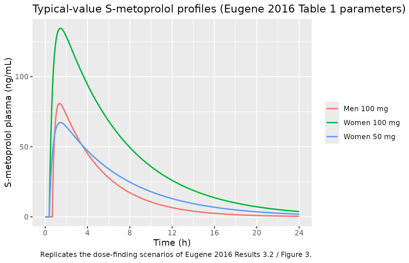
The Women 50 mg curve sits essentially on top of a halved Women 100 mg curve and reaches the same total exposure as Men 100 mg – that superposition is the paper’s conclusion.

conc_obj <- PKNCA::PKNCAconc(
  sim_enant |> filter(!is.na(Cc_s_enant)) |> select(id, time, Cc_s_enant, treatment) |> as.data.frame(),
  Cc_s_enant ~ time | treatment + id,
  concu = "ng/mL", timeu = "hr"
)

dose_obj <- PKNCA::PKNCAdose(
  events_enant |> filter(evid == 1) |> select(id, time, amt, treatment) |> as.data.frame(),
  amt ~ time | treatment + id,
  doseu = "mg"
)

intervals <- data.frame(
  start = 0, end = 24,
  cmax = TRUE, tmax = TRUE, auclast = TRUE, aucinf.obs = TRUE, half.life = TRUE
)

nca_res <- suppressMessages(suppressWarnings(
  PKNCA::pk.nca(PKNCA::PKNCAdata(conc_obj, dose_obj, intervals = intervals))
))

nca_wide <- as.data.frame(nca_res) |>
  select(treatment, PPTESTCD, PPORRES) |>
  tidyr::pivot_wider(names_from = PPTESTCD, values_from = PPORRES)

nca_wide |>
  mutate(across(where(is.numeric), ~ signif(.x, 4))) |>
  knitr::kable(caption = "PKNCA results from the simulated typical-value profiles.")

PKNCA results from the simulated typical-value profiles.
treatment	auclast	cmax	tmax	tlast	clast.obs	lambda.z	r.squared	adj.r.squared	lambda.z.time.first	lambda.z.time.last	lambda.z.n.points	clast.pred	half.life	span.ratio	aucinf.obs
Men 100 mg	393.7	80.87	1.35	24	0.3636	0.2405	0.9999	0.9999	1.36	24	321	0.3659	2.882	7.855	395.3
Women 100 mg	966.7	134.50	1.44	24	3.7650	0.1604	0.9999	0.9999	1.61	24	296	3.7900	4.320	5.183	990.2
Women 50 mg	483.4	67.23	1.44	24	1.8830	0.1604	0.9999	0.9999	1.61	24	296	1.8950	4.320	5.183	495.1

simulated <- nca_wide |>
  transmute(
    treatment,
    Cmax = cmax,
    Tmax = tmax,
    `AUC0-24` = auclast,
    `t-half` = half.life
  )

# Eugene 2016 Results 3.2, verbatim.
reference <- tribble(
  ~treatment,      ~Cmax,  ~Tmax, ~`AUC0-24`, ~`t-half`,
  "Men 100 mg",    80.9,   1.35,  394,        2.9,
  "Women 100 mg",  134.5,  1.44,  967,        4.3,
  "Women 50 mg",   67.2,   1.44,  483,        4.3
) |>
  mutate(treatment = factor(treatment, levels = levels(arms$treatment)))

nlmixr2lib::ncaComparisonTable(
  simulated = simulated,
  reference = reference,
  by = "treatment",
  units = c(Cmax = "ng/mL", Tmax = "h", `AUC0-24` = "ng*h/mL", `t-half` = "h"),
  label_first_column = "NCA parameter"
) |>
  knitr::kable(caption = "Simulated NCA vs Eugene 2016 Results 3.2 (published values verbatim).")
#> Warning: ncaParamLabel(): unknown PKNCA code(s) returned as-is: 'Cmax', 'Tmax',
#> 'AUC0-24', 't-half'

Simulated NCA vs Eugene 2016 Results 3.2 (published values verbatim).
NCA parameter	treatment	Reference	Simulated	% diff
AUC0-24 (ng*h/mL)	Men 100 mg	394	394	-0.1%
AUC0-24 (ng*h/mL)	Women 100 mg	967	967	-0.0%
AUC0-24 (ng*h/mL)	Women 50 mg	483	483	+0.1%
Cmax (ng/mL)	Men 100 mg	80.9	80.9	-0.0%
Cmax (ng/mL)	Women 100 mg	134	134	-0.0%
Cmax (ng/mL)	Women 50 mg	67.2	67.2	+0.0%
t-half (h)	Men 100 mg	2.9	2.88	-0.6%
t-half (h)	Women 100 mg	4.3	4.32	+0.5%
t-half (h)	Women 50 mg	4.3	4.32	+0.5%
Tmax (h)	Men 100 mg	1.35	1.35	+0.0%
Tmax (h)	Women 100 mg	1.44	1.44	+0.0%
Tmax (h)	Women 50 mg	1.44	1.44	+0.0%

cmp <- simulated |>
  rename(Cmax_sim = Cmax, Tmax_sim = Tmax, AUC_sim = `AUC0-24`, thalf_sim = `t-half`) |>
  left_join(
    reference |> rename(Cmax_pub = Cmax, Tmax_pub = Tmax, AUC_pub = `AUC0-24`, thalf_pub = `t-half`),
    by = "treatment"
  )

knitr::kable(cmp |> mutate(across(where(is.numeric), ~ signif(.x, 4))),
  caption = "Side-by-side values entering the assertions below.")

Side-by-side values entering the assertions below.
treatment	Cmax_sim	Tmax_sim	AUC_sim	thalf_sim	Cmax_pub	Tmax_pub	AUC_pub	thalf_pub
Men 100 mg	80.87	1.35	393.7	2.882	80.9	1.35	394	2.9
Women 100 mg	134.50	1.44	966.7	4.320	134.5	1.44	967	4.3
Women 50 mg	67.23	1.44	483.4	4.320	67.2	1.44	483	4.3


# These two sides do NOT differ by a physical per-subject mechanism: both are
# deterministic typical-value solves of the same parameter set, so the only
# difference is numerical quadrature plus the paper's own rounding. Tight
# absolute bounds are therefore correct here (see the package CLAUDE.md note on
# vignette assertions -- the loose-quantile rule applies to random cohorts).
#
# Tolerances are half of the last printed digit, widened by the observation
# grid spacing where that is coarser (Tmax can only be resolved to 0.01 h).
stopifnot(
  max(abs(cmp$Cmax_sim - cmp$Cmax_pub)) < 0.5, # ng/mL; published to 3 s.f.
  max(abs(cmp$Tmax_sim - cmp$Tmax_pub)) < 0.02, # h; grid resolution 0.01 h
  max(abs(cmp$thalf_sim - cmp$thalf_pub)) < 0.1, # h; published to 2 s.f.
  max(abs(cmp$AUC_sim - cmp$AUC_pub) / cmp$AUC_pub) < 0.01 # AUC within 1%
)

Independent closed-form gate

aucinf.obs for a one-compartment oral model with complete input must equal Dose / (CL/F) exactly. This gate is independent of the NCA quadrature and catches a mis-scaled dose, a wrong volume, or a lost unit conversion.

auc_gate <- nca_wide |>
  left_join(arms |> select(treatment, dose, SEXF), by = "treatment") |>
  mutate(
    cl_pub = if_else(SEXF == 0, 253, 101),
    auc_closed_form = 1000 * dose / cl_pub,
    pct_diff = 100 * (aucinf.obs - auc_closed_form) / auc_closed_form
  ) |>
  select(treatment, dose, cl_pub, aucinf.obs, auc_closed_form, pct_diff)

auc_gate |>
  mutate(across(where(is.numeric), ~ signif(.x, 5))) |>
  rename("Treatment" = treatment, "Dose (mg)" = dose, "Published CL/F (L/h)" = cl_pub,
    "AUCinf simulated" = aucinf.obs, "Dose/CL closed form" = auc_closed_form,
    "Difference (%)" = pct_diff) |>
  knitr::kable(caption = "Mass-balance gate: AUC0-inf must equal Dose / (CL/F).")

Mass-balance gate: AUC0-inf must equal Dose / (CL/F).
Treatment	Dose (mg)	Published CL/F (L/h)	AUCinf simulated	Dose/CL closed form	Difference (%)
Men 100 mg	100	253	395.26	395.26	-0.0001509
Women 100 mg	100	101	990.18	990.10	0.0077666
Women 50 mg	50	101	495.09	495.05	0.0077670


stopifnot(max(abs(auc_gate$pct_diff)) < 0.5)

Dose equivalence – the paper’s conclusion, asserted

auc_by_arm <- setNames(nca_wide$auclast, as.character(nca_wide$treatment))
ratio_5050 <- auc_by_arm[["Women 50 mg"]] / auc_by_arm[["Men 100 mg"]]
ratio_100100 <- auc_by_arm[["Women 100 mg"]] / auc_by_arm[["Men 100 mg"]]

tibble(
  Comparison = c("Women 100 mg vs Men 100 mg", "Women 50 mg vs Men 100 mg"),
  `AUC0-24 ratio` = round(c(ratio_100100, ratio_5050), 3)
) |>
  knitr::kable(caption = "Exposure ratios underpinning the 50 mg / 100 mg dose-equivalence recommendation.")

Exposure ratios underpinning the 50 mg / 100 mg dose-equivalence recommendation.
Comparison	AUC0-24 ratio
Women 100 mg vs Men 100 mg	2.455
Women 50 mg vs Men 100 mg	1.228

At the same 100 mg dose, women reach roughly 2.5-fold the exposure of men, consistent with the Luzier 1999 observation quoted in the Introduction (AUC 867 vs 417 mcg*h/L, a 2.1-fold ratio). Halving the female dose brings the ratio to approximately 1.2 – close to unity, which is the basis for the paper’s recommendation.

# Assert the direction and approximate magnitude of BOTH claims. The 100 mg
# comparison is the paper's motivating observation; the 50 mg comparison is its
# conclusion. Both are deterministic here, so exact-ish bounds are appropriate.
stopifnot(
  ratio_100100 > 2.0, # women substantially over-exposed at an equal dose
  ratio_5050 > 1.0, ratio_5050 < 1.4 # halving the dose brings exposure near parity
)

Note that the match is close but not perfect: the paper describes 50 mg in women as giving “approximately similar” exposure to 100 mg in men, and the residual ~20% over-exposure is visible in the table above. That is a property of the published parameters, not of this encoding – 483 / 394 = 1.23 using the paper’s own Results 3.2 numbers.

R- versus S-metoprolol

Only the Table 1 model carries R-metoprolol; Table 2 dropped it. S-metoprolol is the pharmacologically active enantiomer, which is why the paper’s dose-finding uses it, but the R-enantiomer parameters are reported and are extracted here.

ev_both <- bind_rows(
  arms |> filter(id <= 2) |> mutate(time = 0, amt = dose, evid = 1L, cmt = "depot_s_enant", dvid = NA_integer_),
  arms |> filter(id <= 2) |> mutate(time = 0, amt = dose, evid = 1L, cmt = "depot_r_enant", dvid = NA_integer_),
  arms |> filter(id <= 2) |> tidyr::crossing(time = obs_times) |>
    mutate(amt = NA_real_, evid = 0L, cmt = NA_character_, dvid = 1L),
  arms |> filter(id <= 2) |> tidyr::crossing(time = obs_times) |>
    mutate(amt = NA_real_, evid = 0L, cmt = NA_character_, dvid = 2L)
) |>
  select(id, time, amt, evid, cmt, dvid, SEXF, treatment) |>
  arrange(id, time, desc(evid)) |>
  as.data.frame()

sim_both <- rxode2::rxSolve(rxode2::zeroRe(mod_enant), ev_both,
  keep = c("SEXF", "treatment"), returnType = "data.frame")
#> Warning: No omega parameters in the model
#> Warning: multi-subject simulation without without 'omega'

long_both <- bind_rows(
  sim_both |> filter(!is.na(Cc_r_enant)) |> transmute(time, treatment, Enantiomer = "R", Cc = Cc_r_enant),
  sim_both |> filter(!is.na(Cc_s_enant)) |> transmute(time, treatment, Enantiomer = "S", Cc = Cc_s_enant)
) |>
  distinct(time, treatment, Enantiomer, .keep_all = TRUE)

ggplot(long_both, aes(time, Cc, colour = Enantiomer, linetype = treatment)) +
  geom_line(linewidth = 0.7) +
  scale_x_continuous(breaks = seq(0, 24, by = 4)) +
  labs(
    x = "Time (h)", y = "Plasma concentration (ng/mL)", linetype = NULL,
    title = "R- vs S-metoprolol after a 100 mg dose (Eugene 2016 Table 1)",
    caption = "R-metoprolol has the higher apparent clearance in both sexes, so it reaches lower concentrations."
  )

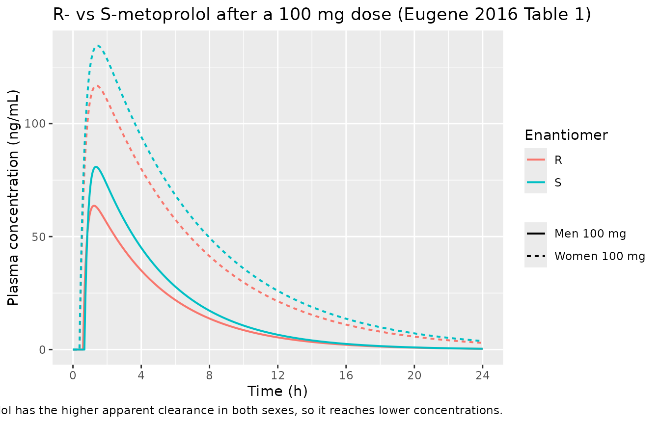
# R-metoprolol has a higher CL/F than S in BOTH sexes (316 vs 253 in men,
# 120 vs 101 in women), so its exposure must be lower in both. This is the
# direction that would silently invert if the R and S columns were transposed.
auc_enant <- long_both |>
  group_by(treatment, Enantiomer) |>
  arrange(time, .by_group = TRUE) |>
  summarise(auc = sum(diff(time) * (head(Cc, -1) + tail(Cc, -1)) / 2), .groups = "drop") |>
  tidyr::pivot_wider(names_from = Enantiomer, values_from = auc)

auc_enant |>
  mutate(ratio_R_over_S = round(R / S, 3), across(where(is.numeric), ~ signif(.x, 4))) |>
  knitr::kable(caption = "AUC0-24 by enantiomer; R/S ratio should track the inverse clearance ratio.")

AUC0-24 by enantiomer; R/S ratio should track the inverse clearance ratio.
treatment	R	S	ratio_R_over_S
Men 100 mg	315.1	393.8	0.800
Women 100 mg	815.6	966.8	0.844


stopifnot(all(auc_enant$R < auc_enant$S))
# Dose/CL predicts the ratio: men 253/316 = 0.80, women 101/120 = 0.84.
stopifnot(
  abs(auc_enant$R[auc_enant$treatment == "Men 100 mg"] /
    auc_enant$S[auc_enant$treatment == "Men 100 mg"] - 253 / 316) < 0.02,
  abs(auc_enant$R[auc_enant$treatment == "Women 100 mg"] /
    auc_enant$S[auc_enant$treatment == "Women 100 mg"] - 101 / 120) < 0.02
)

Part 2 – The Table 2 Clinical Trial Simulation model

Table 2 is a re-estimate from the paper’s own simulated dataset (Methods 2.4): 50 men and 50 women, each given 100 mg of S-metoprolol and sampled at 17 fixed times, giving 1700 plasma samples. Because the simulation injected per-subject variability, the re-fit recovers inter-individual variance terms that Table 1 does not have.

Structural parameter recovery

tbl2 <- tribble(
  ~SEXF, ~tlag,  ~ka,    ~vc,   ~cl,
  0,     0.677,  0.233,  49,    231,
  1,     0.38,   0.149,  33.3,  92.9
)

probe_cts <- function(sexf) {
  ev <- bind_rows(
    tibble(id = 1L, time = 0, amt = 100, evid = 1L, cmt = "depot"),
    tibble(id = 1L, time = c(0, 1), amt = NA_real_, evid = 0L, cmt = "central")
  )
  rxode2::rxSolve(rxode2::zeroRe(mod_cts), ev, params = c(SEXF = as.numeric(sexf)),
    returnType = "data.frame")[1, ]
}

chk2 <- bind_rows(lapply(c(0, 1), function(sx) {
  p <- probe_cts(sx)
  tibble(SEXF = sx, tlag = p$tlag, ka = p$ka, vc = p$vc, cl = p$cl)
})) |>
  right_join(tbl2, by = "SEXF", suffix = c("_sim", "_pub"))
#> ℹ omega/sigma items treated as zero: 'etaltlag', 'etalka', 'etalvc', 'etalcl'
#> ℹ omega/sigma items treated as zero: 'etaltlag', 'etalka', 'etalvc', 'etalcl'

chk2 |>
  mutate(across(where(is.numeric), ~ signif(.x, 4))) |>
  knitr::kable(caption = "Eugene 2016 Table 2 (published) vs recovered from the model file.")

Eugene 2016 Table 2 (published) vs recovered from the model file.
SEXF	tlag_sim	ka_sim	vc_sim	cl_sim	tlag_pub	ka_pub	vc_pub	cl_pub
0	0.677	0.233	49.0	231.0	0.677	0.233	49.0	231.0
1	0.380	0.149	33.3	92.9	0.380	0.149	33.3	92.9


stopifnot(
  max(abs(chk2$tlag_pub - chk2$tlag_sim)) < 1e-8,
  max(abs(chk2$ka_pub - chk2$ka_sim)) < 1e-8,
  max(abs(chk2$vc_pub - chk2$vc_sim)) < 1e-8,
  max(abs(chk2$cl_pub - chk2$cl_sim)) < 1e-8
)

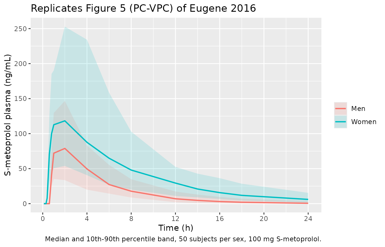
Reproducing the Clinical Trial Simulation (Figures 4 and 5)

The cohort below matches the paper’s design exactly: 50 men + 50 women, 100 mg, at the 17 sample times listed in Methods 2.4.

n_per_sex <- 50 # exactly the paper's design; well under the 200-per-arm cap

cts_times <- c(0, 0.1, 0.2, 0.3, 0.4, 0.6, 0.8, 1, 2, 4, 6, 8, 12, 14, 16, 18, 24)

cts_cohort <- tibble(
  id = seq_len(2 * n_per_sex),
  SEXF = rep(c(0, 1), each = n_per_sex)
) |>
  mutate(treatment = factor(if_else(SEXF == 1, "Women", "Men"), levels = c("Men", "Women")))

cts_events <- bind_rows(
  cts_cohort |> mutate(time = 0, amt = 100, evid = 1L, cmt = "depot"),
  cts_cohort |> tidyr::crossing(time = cts_times) |>
    mutate(amt = NA_real_, evid = 0L, cmt = "central")
) |>
  select(id, time, amt, evid, cmt, SEXF, treatment) |>
  arrange(id, time, desc(evid)) |>
  as.data.frame()

sim_cts <- rxode2::rxSolve(mod_cts, cts_events, keep = c("SEXF", "treatment"),
  returnType = "data.frame")

# The paper states the CTS produced 1700 plasma samples (850 per sex).
n_samples <- sum(!is.na(sim_cts$Cc))
stopifnot(n_samples == 1700L)

1700 simulated plasma samples, matching the 1700 stated in Results 3.3.

vpc <- sim_cts |>
  filter(!is.na(Cc), time > 0) |>
  group_by(time, treatment) |>
  summarise(
    Q10 = quantile(Cc, 0.10), Q50 = quantile(Cc, 0.50), Q90 = quantile(Cc, 0.90),
    .groups = "drop"
  )

ggplot(vpc, aes(time, Q50, colour = treatment, fill = treatment)) +
  geom_ribbon(aes(ymin = Q10, ymax = Q90), alpha = 0.15, colour = NA) +
  geom_line(linewidth = 0.8) +
  scale_x_continuous(breaks = seq(0, 24, by = 4)) +
  labs(
    x = "Time (h)", y = "S-metoprolol plasma (ng/mL)", colour = NULL, fill = NULL,
    title = "Replicates Figure 5 (PC-VPC) of Eugene 2016",
    caption = sprintf("Median and 10th-90th percentile band, %d subjects per sex, 100 mg S-metoprolol.", n_per_sex)
  )

# Cohort-level assertions. Per the package CLAUDE.md guidance these are stated
# on the CENTRE and on robust quantiles -- never on the per-subject extreme,
# which is not reproducible across rxode2 builds.
exposure <- sim_cts |>
  filter(!is.na(Cc)) |>
  group_by(id, treatment) |>
  arrange(time, .by_group = TRUE) |>
  summarise(auc = sum(diff(time) * (head(Cc, -1) + tail(Cc, -1)) / 2), .groups = "drop")

med_auc <- exposure |> group_by(treatment) |> summarise(med = median(auc), .groups = "drop")

knitr::kable(med_auc |> mutate(med = signif(med, 4)) |>
  rename("Treatment" = treatment, "Median AUC0-24 (ng*h/mL)" = med),
caption = "Median per-subject exposure in the simulated cohort.")

Median per-subject exposure in the simulated cohort.
Treatment	Median AUC0-24 (ng*h/mL)
Men	444.9
Women	970.6


ratio_cts <- med_auc$med[med_auc$treatment == "Women"] /
  med_auc$med[med_auc$treatment == "Men"]

# Structural: the typical-value AUC ratio is 231/92.9 = 2.49. The cohort median
# must land near it; a mis-transcribed CL or a dropped sex effect moves this by
# tens of percent. The band is wide enough to absorb the sampling noise of a
# 50-per-arm median but far tighter than any transcription error.
stopifnot(ratio_cts > 1.9, ratio_cts < 3.2)

# Every subject's exposure must be positive and finite -- catches a lost lag
# time or a zeroed depot.
stopifnot(all(is.finite(exposure$auc)), all(exposure$auc > 0))

cts_conc <- PKNCA::PKNCAconc(
  sim_cts |> filter(!is.na(Cc)) |> select(id, time, Cc, treatment) |> as.data.frame(),
  Cc ~ time | treatment + id, concu = "ng/mL", timeu = "hr"
)
cts_dose <- PKNCA::PKNCAdose(
  cts_events |> filter(evid == 1) |> select(id, time, amt, treatment) |> as.data.frame(),
  amt ~ time | treatment + id, doseu = "mg"
)

cts_nca <- suppressMessages(suppressWarnings(PKNCA::pk.nca(
  PKNCA::PKNCAdata(cts_conc, cts_dose,
    intervals = data.frame(start = 0, end = 24, cmax = TRUE, tmax = TRUE, auclast = TRUE))
)))

summary(cts_nca) |>
  knitr::kable(caption = "Cohort NCA summary for the Table 2 CTS model (median and 5th-95th percentiles).")

Cohort NCA summary for the Table 2 CTS model (median and 5th-95th percentiles).
Interval Start	Interval End	treatment	N	AUClast (hr*ng/mL)	Cmax (ng/mL)	Tmax (hr)
0	24	Men	50	431 [60.3]	83.3 [67.5]	2.00 [0.800, 2.00]
0	24	Women	50	946 [57.3]	119 [68.5]	2.00 [0.600, 2.00]

The Table 2 model’s typical-value exposures sit systematically above the Table 1 values (Dose/CL = 433 vs 395 ng*h/mL in men, 1076 vs 990 in women) because the CTS re-fit recovered a slightly lower clearance than the original fit. The paper’s published NCA table (Results 3.2) comes from Table 1, so the Table 1 model is the one validated against it above.

Assumptions and deviations

Two model files from one paper. Table 1 and Table 2 are different estimates, from different datasets, with different analyte scope. Rather than pick one, both are extracted per the library’s replicate-the-author’s-structure policy. Table 2 is the only one with random effects; Table 1 is the only one with R-metoprolol and the only one that reproduces the paper’s published NCA.
Sex encoded with male as the reference. Neither Table 1 nor Table 2 publishes a covariate coefficient – each prints a male column and a female column outright. The canonical SEXF column (1 = female, 0 = male) is used, with the male value as the structural reference and each e_sexf_* term computed as log(female / male). This is an exact re-parameterisation: the structural-recovery checks above confirm both published columns are returned verbatim. No sex-difference information is added or lost.
No residual error is reported for the Table 1 model, so propSd_r_enant and propSd_s_enant are fixed(0) rather than invented. This is faithful: Table 1 was fit to digitized mean curves, not to individual observations, so there is no within-subject residual to report. Simulating from that model returns typical-value profiles.
No inter-individual variability is reported for the Table 1 model either, for the same reason. Users who need a stochastic S-metoprolol cohort should use Eugene_2016b_metoprolol (Table 2), which has the variance terms.
The Table 2 omega values are variances on the log scale. Table 2’s CV(%) column is MONOLIX’s log-scale SD, which equals sqrt(omega^2) – sqrt(0.176) = 42.0% against a printed 42% for Ka, sqrt(0.182) = 42.7% against 43% for V, and sqrt(0.305) = 55.2% against 55% for CL. The variances are entered verbatim.
omega^2 for Tlag is effectively unidentified. Table 2 reports 0.0003 with an SE of 0.0021 – an RSE of 809%, larger than the estimate by a factor of seven. It is entered as published, but it should be read as “no detectable variability in lag time”, not as a meaningful estimate. Its printed CV of 0.20% is also inconsistent with sqrt(0.0003) = 1.7%, unlike the other three rows which reconcile exactly; nothing in the paper resolves that discrepancy.
Table 2 parameters are estimated from simulated, not observed, data. The CTS drew subjects using Table 1 typical values plus per-sex CVs carried over from Luzier 1999, then re-fit that synthetic dataset. The recovered variabilities are therefore close to the assumed inputs by construction (CL 55% recovered vs 59%/49% assumed; V 43% vs 44%/34%; Ka 42% vs an assumed 40%). They characterise the paper’s simulation, not a real population.
Flip-flop kinetics are a derived finding, not a stated one. The paper never remarks that absorption is rate-limiting, but its own numbers require it: the reported half-lives of 2.9 h and 4.3 h equal ln(2)/Ka, while ln(2)/(CL/V) is about nine minutes. Any downstream user who assumes the terminal slope is elimination will mis-scale this model, so it is asserted explicitly above.
Body weight is not in the model. Eugene 2016 discusses the 21 kg mean weight difference between the male and female Luzier cohorts as a likely driver of the exposure difference, but does not include weight as a covariate. The sex effect therefore absorbs whatever part of the difference is really due to body size, and the model should not be extrapolated across weights within a sex.
The dose amount is the full administered dose for each enantiomer. Table 1 and Table 2 CL/F values were fit against the full 100 mg, not against 50 mg of each enantiomer from the racemate: 100 mg / 253 L/h = 395 ngh/mL reproduces the published 394 ngh/mL for men. Dose each depot with the full dose amount, as the closed-form gate above verifies.
Observed data are not redistributed. The digitized Luzier 1999 curves are not public, so this vignette validates against the paper’s published numeric summaries rather than overlaying observations.