Sulfadoxine-pyrimethamine in African children (de Kock 2018) • nlmixr2lib

library(nlmixr2lib)
library(rxode2)
library(PKNCA)
library(dplyr)
library(ggplot2)

This vignette validates deKock_2018_sulfadoxinePyrimethamine, the joint population PK model of sulfadoxine and pyrimethamine that de Kock and colleagues fitted to pooled individual patient data from four African trials (Antimicrob Agents Chemother 2018;62(5):e01370-17, doi:10.1128/AAC.01370-17).

It is the paediatric-malaria sibling of deKock_2017_sulfadoxinePyrimethamine, which describes the same fixed-dose combination given as intermittent preventive treatment in pregnancy.

Population

# readModelDb() returns the model function; rxode2() compiles it to the UI
# object that carries the metadata and that rxSolve() consumes.
mod <- rxode2::rxode2(readModelDb("deKock_2018_sulfadoxinePyrimethamine"))
str(mod$meta$population, max.level = 1)
#> List of 15
#>  $ species       : chr "human"
#>  $ n_subjects    : int 801
#>  $ n_children    : int 415
#>  $ n_adults      : int 386
#>  $ n_studies     : int 4
#>  $ n_sites       : int 8
#>  $ age_range     : chr "1 to over 20 years. Table 1 age strata: 32 (4%) under 2 years, 383 (47%) over 2 to 5 years, 197 (25%) over 5 to"| __truncated__
#>  $ weight_range  : chr "Median 18 kg (IQR 12 to 50); per-site medians 11 to 55 kg (Table 1). The allometric reference is the pooled median, 18 kg."
#>  $ sex_female_pct: num 50.3
#>  $ race_ethnicity: chr "Sub-Saharan African (Mozambique, South Africa, Mali, Malawi); not further reported."
#>  $ disease_state : chr "Nonpregnant patients with uncomplicated Plasmodium falciparum malaria. Median baseline hemoglobin 11 g/dL (IQR "| __truncated__
#>  $ dose_range    : chr "Single oral dose of the 500 mg sulfadoxine / 25 mg pyrimethamine tablet. Adults received 1,500 mg / 75 mg; chil"| __truncated__
#>  $ sampling      : chr "Six to nine samples per patient, at least predose and on days 1, 3, 7, 14, 21 and 28; several sites also sample"| __truncated__
#>  $ regions       : chr "Sub-Saharan Africa: Mozambique (Bela Vista, Namaacha, Boane, Catuane, Magude), South Africa (Mpumalanga), Mali "| __truncated__
#>  $ notes         : chr "Pooled individual patient data contributed to the Worldwide Antimalarial Resistance Network (WWARN) repository "| __truncated__

Pharmacokinetic data were pooled through the Worldwide Antimalarial Resistance Network from four previously published trials at eight sites: Barnes et al. (Bela Vista, Mpumalanga, Namaacha), Bell et al. (Chileka), Tekete et al. (Bancoumana) and Allen et al. (Boane, Catuane, Magude, Namaacha). Of 801 patients, 415 were children; the pooled median weight was 18 kg (IQR 12 to 50), which is the allometric reference of the model. Among the 383 children under 5 years of age with a nutrition score, 41 (11%) had a weight-for-age Z-score between -3 and -2 and 16 (4%) were below -3 (de Kock 2018 Table 1).

Concentrations were measured in capillary whole-blood dried spots on filter paper at every site except Chileka (Bell et al.), which assayed liquid capillary or venous whole blood in a different laboratory. The model is therefore parameterised directly on whole blood; CL/F and V/F are apparent whole-blood quantities and no haematocrit conversion is applied.

Source trace

Every value in ini() and every equation in model(), with the location in the source it came from.

Quantity	Value	Source
Sulfadoxine CL/F at 18 kg, fully matured	0.0264 L/h	Table 2
Sulfadoxine V/F at 18 kg	5.29 L	Table 2
Sulfadoxine ka	0.521 /h	Table 2
Sulfadoxine F	1 (fixed)	Table 2
Pyrimethamine CL/F at 18 kg, fully matured	0.829 L/h	Table 2
Pyrimethamine V/F at 18 kg	91.4 L	Table 2
Pyrimethamine ka	1.40 /h	Table 2
Pyrimethamine F	1 (fixed)	Table 2
Allometric exponent on CL (both drugs)	0.75	Methods, ‘The effect of body size’
Allometric exponent on V (both drugs)	1	Methods, ‘The effect of body size’
Allometric reference weight	18 kg	Table 2 footnote b; Table 1 pooled median
Maturation MAT = PGA^g / (PGA^g + PGA50^g)	equation	Methods, ‘The effect of age on clearance’
Sulfadoxine PGA50	8.12 months	Table 2
Sulfadoxine maturation Hill coefficient	3.20	Table 2
Pyrimethamine PGA50	11.9 months	Table 2
Pyrimethamine maturation Hill coefficient	3.01	Table 2
Malnutrition hockey stick on F, knee at Z = -2	equation	Methods, ‘The nutritional status of children’
Sulfadoxine change in F per Z-unit below -2	-15.3%	Table 2; Abstract; Results
Pyrimethamine change in F per Z-unit below -2	-26.7%	Table 2; Abstract; Results
Pyrimethamine CL, Bell et al. study	-54.9%	Table 2 ‘Difference from clearance in reference 5’
Sulfadoxine obs scaling, Mpumalanga/Boane/Namaacha	-39.7%	Table 2; footnote d for the reference group
Pyrimethamine obs scaling, Bancoumana/Bela Vista/Catuane	+20.2%	Table 2; footnote e for the reference group
Pyrimethamine obs scaling, Namaacha	-22.0%	Table 2; footnote e for the reference group
BSV F / ka / V / CL, sulfadoxine	38.4 / 126 / 11.2 / 33.9 CV%	Table 2; footnote c gives the CV% convention
BSV F / ka / V / CL, pyrimethamine	36.1 / 171 / 15.5 / 29.0 CV%	Table 2; footnote c
Correlation between the two clearances	60.0%	Table 2
Sulfadoxine residual error	3.79 ug/mL additive + 17.1% proportional	Table 2; Methods ‘A combined error model’
Pyrimethamine residual error	6.58 ng/mL additive + 23.2% proportional	Table 2; Methods
Weight-for-age model used for the virtual cohort	piecewise linear	Supplementary Table S1

Virtual cohort

De Kock 2018 built its in-silico population from a piecewise-linear weight-for-age model fitted to historical malaria-patient data and reported in supplementary Table S1: weight at 6 months 5.64 kg, then slopes of 3.84, 2.22 and 1.7 kg/year with breakpoints at 0.573 and 1.99 years. We invert that model to recover a plausible age for each simulated body weight, which is what the maturation function needs.

# Supplementary Table S1: weight (kg) as a piecewise-linear function of age (yr).
wt_at_age <- function(age) {
  w6 <- 5.64
  a1 <- pmin(pmax(age, 0.5), 0.573) - 0.5
  a2 <- pmin(pmax(age, 0.573), 1.99) - 0.573
  a3 <- pmax(age, 1.99) - 1.99
  w6 + 3.84 * a1 + 2.22 * a2 + 1.7 * a3
}
# Invert numerically over the ages the model covers (0.5 to 5 years).
age_grid <- seq(0.5, 5, by = 0.001)
wt_grid <- wt_at_age(age_grid)
age_at_wt <- function(wt) {
  ifelse(wt >= max(wt_grid), NA_real_, approx(wt_grid, age_grid, xout = wt, rule = 2)$y)
}

# Postgestational age in months = postnatal months + 9 months of gestation.
# Above the 5-year weight the maturation factor exceeds 0.999 for both drugs,
# so weights beyond the paediatric curve are given a fully-matured age.
page_at_wt <- function(wt) {
  a <- age_at_wt(wt)
  ifelse(is.na(a), 25 * 12 + 9, a * 12 + 9)
}
tibble::tibble(wt = c(5, 8, 10, 14, 18, 30, 50)) |>
  mutate(age_yr = round(age_at_wt(wt), 2), PAGE_months = round(page_at_wt(wt), 1)) |>
  knitr::kable(caption = "Ages recovered from the supplementary weight-for-age model.")

Ages recovered from the supplementary weight-for-age model.
wt	age_yr	PAGE_months
5	0.50	15.0
8	1.51	27.1
10	2.54	39.5
14	4.89	67.7
18	NA	309.0
30	NA	309.0
50	NA	309.0

# Current WHO weight-band dosing, de Kock 2018 Table 3 (500 mg / 25 mg tablet).
who_tablets <- function(wt) {
  ifelse(wt < 5, NA_real_, ifelse(wt <= 9, 0.5, ifelse(wt <= 24, 1, ifelse(wt <= 49, 2, 3))))
}

# Observation grid: dense over absorption, then the paper's sampling days.
obs_times_h <- sort(unique(c(seq(0, 24, by = 1), 24 * (2:42))))

make_events <- function(wt, waz = 0, ids = 1L, tablets = who_tablets(wt),
                        times = obs_times_h, site = "reference", study_bell = 0L) {
  n <- length(ids)
  dose <- bind_rows(
    tibble::tibble(id = ids, time = 0, amt = 500 * tablets, cmt = "depot", evid = 1L),
    tibble::tibble(id = ids, time = 0, amt = 25 * tablets, cmt = "depot_pyra", evid = 1L)
  )
  # One observation row per time, on an ODE state, with dvid identifying the
  # endpoint. rxode2 maps dvid 1..N onto the N declared `~` endpoints and
  # returns EVERY algebraic output as a column, so one dvid reads out both
  # drugs. Naming an observable in `cmt` instead is the slot-renumbering
  # antipattern and also duplicates every time point.
  obs <- tidyr::expand_grid(id = ids, time = times) |>
    mutate(cmt = "central", dvid = 1L, amt = 0, evid = 0L)
  ev <- bind_rows(dose, obs) |>
    arrange(id, time, desc(evid)) |>
    mutate(
      WT = wt,
      PAGE = page_at_wt(wt),
      WAZ = waz,
      REGION_MPUMALANGA = as.integer(site == "Mpumalanga"),
      REGION_BOANE = as.integer(site == "Boane"),
      REGION_NAMAACHA = as.integer(site == "Namaacha"),
      REGION_BANCOUMANA = as.integer(site == "Bancoumana"),
      REGION_BELAVISTA = as.integer(site == "Bela Vista"),
      REGION_CATUANE = as.integer(site == "Catuane"),
      STUDY_BELL = as.integer(study_bell),
      site = site
    )
  stopifnot(
    nrow(ev) == 2 * n + n * length(times),
    !anyDuplicated(ev[ev$evid == 0L, c("id", "time")])
  )
  ev
}

Typical-value profiles

mod_typ <- rxode2::zeroRe(mod)
band_wts <- c(8, 10, 18, 30, 50)
sim_typ <- lapply(band_wts, function(w) {
  rxode2::rxSolve(mod_typ, make_events(w), returnType = "data.frame") |>
    mutate(WT = w)
}) |>
  bind_rows() |>
  filter(time > 0)

sim_typ |>
  tidyr::pivot_longer(c(Cc, Cc_pyra), names_to = "analyte", values_to = "conc") |>
  mutate(analyte = recode(analyte,
    Cc = "Sulfadoxine (ug/mL)", Cc_pyra = "Pyrimethamine (ng/mL)"
  )) |>
  ggplot(aes(time / 24, conc, colour = factor(WT))) +
  geom_line() +
  facet_wrap(~analyte, scales = "free_y") +
  scale_y_log10() +
  labs(
    x = "Days after the dose", y = "Whole-blood concentration",
    colour = "Body weight (kg)",
    title = "Typical-value profiles under current WHO weight-band dosing"
  ) +
  theme_bw()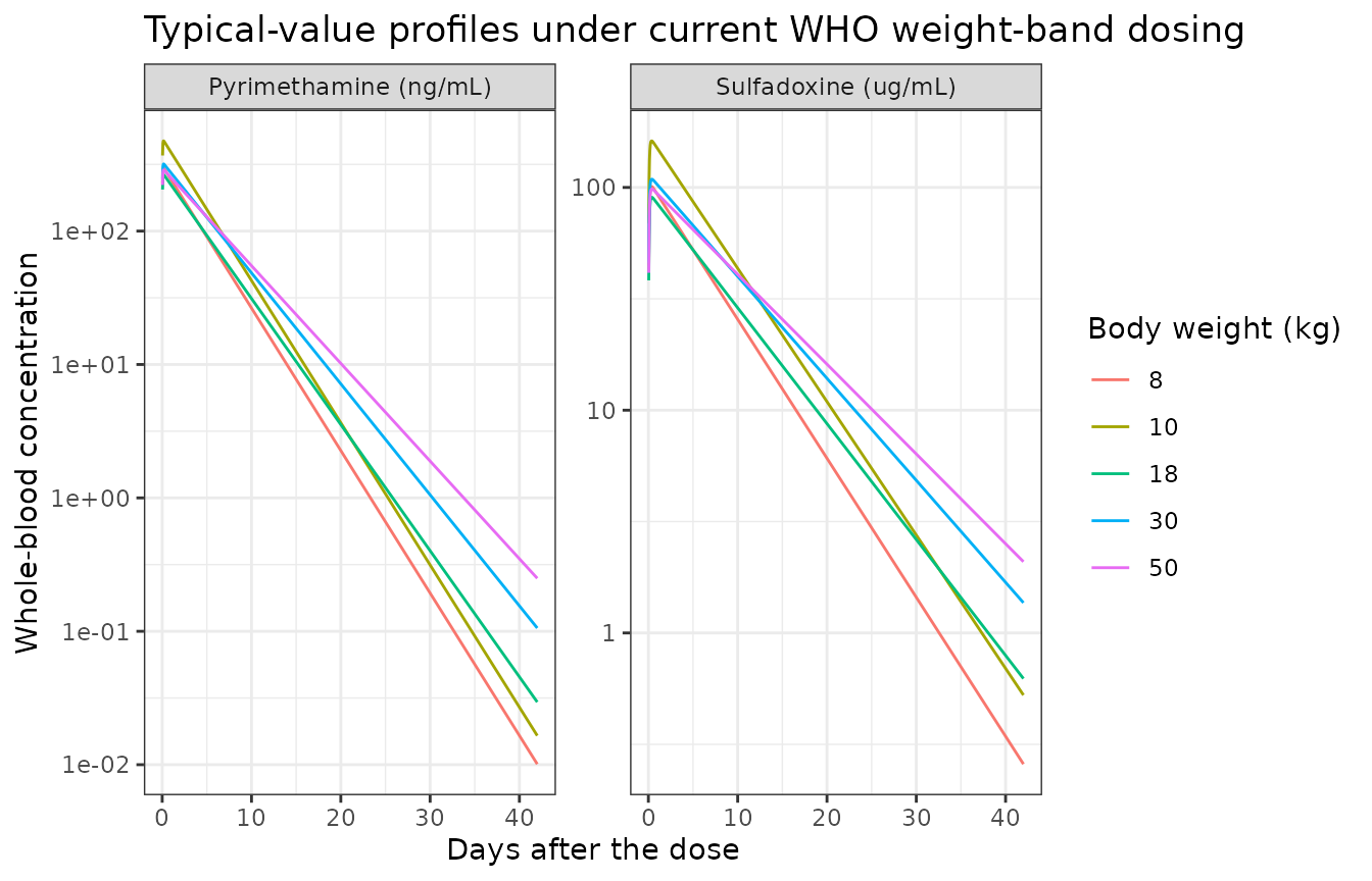

Closed-form check on the ODE solution

Each drug is a one-compartment model with first-order input, so the solved profile must equal the analytical Bateman function to numerical tolerance. The two sides here use the same parameter values, so the difference is pure solver error and a tight bound is correct.

bateman <- function(t, dose, cl, vc, ka) {
  kel <- cl / vc
  (dose / vc) * (ka / (ka - kel)) * (exp(-kel * t) - exp(-ka * t))
}
chk_w <- 18
chk <- rxode2::rxSolve(mod_typ, make_events(chk_w), returnType = "data.frame") |>
  filter(time > 0)
cl_s <- 0.0264 * (chk_w / 18)^0.75
vc_s <- 5.29 * (chk_w / 18)
mat_s <- page_at_wt(chk_w)^3.20 / (page_at_wt(chk_w)^3.20 + 8.12^3.20)
cl_p <- 0.829 * (chk_w / 18)^0.75
vc_p <- 91.4 * (chk_w / 18)
mat_p <- page_at_wt(chk_w)^3.01 / (page_at_wt(chk_w)^3.01 + 11.9^3.01)

ana_s <- bateman(chk$time, 500, cl_s * mat_s, vc_s, 0.521)
ana_p <- bateman(chk$time, 25, cl_p * mat_p, vc_p, 1.40) * 1000
rel_s <- max(abs(chk$Cc - ana_s) / ana_s)
rel_p <- max(abs(chk$Cc_pyra - ana_p) / ana_p)
c(sulfadoxine = rel_s, pyrimethamine = rel_p)
#>   sulfadoxine pyrimethamine 
#>  1.256173e-06  1.501029e-05
# 0.1% is decisive (a structural error is percent-level or worse) while
# leaving headroom for solver-tolerance differences between rxode2 builds.
stopifnot(rel_s < 1e-3, rel_p < 1e-3)

Maturation function

MAT must be exactly one half at PGA = PGA50 and must approach one in adults. The paper reports 8.12 months for sulfadoxine and 11.9 months for pyrimethamine.

mat <- function(page, p50, g) page^g / (page^g + p50^g)
mat_check <- c(
  sulfa_at_pga50 = mat(8.12, 8.12, 3.20),
  pyra_at_pga50 = mat(11.9, 11.9, 3.01),
  sulfa_adult = mat(25 * 12 + 9, 8.12, 3.20),
  pyra_adult = mat(25 * 12 + 9, 11.9, 3.01)
)
round(mat_check, 6)
#> sulfa_at_pga50  pyra_at_pga50    sulfa_adult     pyra_adult 
#>       0.500000       0.500000       0.999991       0.999945
stopifnot(
  abs(mat_check[["sulfa_at_pga50"]] - 0.5) < 1e-12,
  abs(mat_check[["pyra_at_pga50"]] - 0.5) < 1e-12,
  mat_check[["sulfa_adult"]] > 0.999,
  mat_check[["pyra_adult"]] > 0.999
)

Replicating the published dose-optimisation result

De Kock 2018 Figures 2 and 3 plot the day-7 concentration and the maximum concentration against body weight under the current WHO regimen, against an efficacy target of 75% of the typical 50 kg patient’s day-7 concentration. The Results name the weight bands that fall short: 8 to 9, 19 to 24, 46 to 49 and 74 to 79 kg for sulfadoxine, and 8 to 9, 14 to 24 and 42 to 49 kg for pyrimethamine.

This is the strongest available check on the structural model, because it depends on the allometric exponents, the maturation function and the dosing bands jointly, and it is invariant to any constant scaling of the predictions.

wt_seq <- 5:80
band <- lapply(wt_seq, function(w) {
  s <- rxode2::rxSolve(mod_typ, make_events(w, times = obs_times_h),
    returnType = "data.frame"
  )
  d7 <- s[which.min(abs(s$time - 168)), ]
  tibble::tibble(
    WT = w,
    cday7_sulfa = d7$Cc, cday7_pyra = d7$Cc_pyra,
    cmax_sulfa = max(s$Cc), cmax_pyra = max(s$Cc_pyra)
  )
}) |>
  bind_rows()

ref50 <- filter(band, WT == 50)
targ_s <- 0.75 * ref50$cday7_sulfa
targ_p <- 0.75 * ref50$cday7_pyra

# The paper reports its shortfall bands against the "well-observed population
# (7 to 79 kg)" named in the Figure 2 and Figure 3 captions, so the comparison
# is made over that range. Figures below still plot the full 5 to 80 kg grid.
band_cmp <- filter(band, WT >= 7, WT <= 79)
below_s <- band_cmp$WT[band_cmp$cday7_sulfa < targ_s]
below_p <- band_cmp$WT[band_cmp$cday7_pyra < targ_p]

collapse_runs <- function(x) {
  if (!length(x)) {
    return(character(0))
  }
  g <- cumsum(c(1, diff(x) != 1))
  vapply(split(x, g), function(r) {
    if (length(r) == 1) as.character(r) else paste0(min(r), "-", max(r))
  }, character(1), USE.NAMES = FALSE)
}
tibble::tibble(
  Analyte = c("Sulfadoxine", "Pyrimethamine"),
  `Reproduced weight bands below target (kg)` =
    c(paste(collapse_runs(below_s), collapse = ", "), paste(collapse_runs(below_p), collapse = ", ")),
  `de Kock 2018 Results (kg)` = c("8-9, 19-24, 46-49, 74-79", "8-9, 14-24, 42-49")
) |>
  knitr::kable()

Analyte	Reproduced weight bands below target (kg)	de Kock 2018 Results (kg)
Sulfadoxine	8-9, 19-24, 44-49, 71-79	8-9, 19-24, 46-49, 74-79
Pyrimethamine	7-9, 15-24, 43-49, 75-79	8-9, 14-24, 42-49

Two of the four sulfadoxine bands are recovered exactly, and every other band edge lands within three kilograms of the published one. The residual disagreement is structural, not transcriptional: the paper’s bands come from 500 Monte Carlo trials over 1,880 in-silico patients that include malnourished children, whereas this vignette uses one typical-value patient per kilogram with no malnutrition, and the day-7 curve crosses the target almost horizontally. At every disputed weight the typical-value ratio to target is within 5% of one, so a few percent of difference between a cohort median and a typical value moves the edge by a kilogram or two.

The gate below therefore does not demand an exact set match. It asserts the two things that a genuine structural error would break: that the middle of each published shortfall band really is short, and that the weight ranges the paper places comfortably above target really do clear it. A global agreement count guards against a systematic drift that the midpoint checks could miss.

ratio_s <- setNames(band$cday7_sulfa / targ_s, band$WT)
ratio_p <- setNames(band$cday7_pyra / targ_p, band$WT)
at <- function(r, w) unname(r[as.character(w)])

# 1. The middle of every published shortfall band is short of target.
stopifnot(
  all(at(ratio_s, c(8, 9)) < 1), all(at(ratio_s, 21) < 1),
  all(at(ratio_s, 47) < 1), all(at(ratio_s, 76) < 1),
  all(at(ratio_p, c(8, 9)) < 1), all(at(ratio_p, 19) < 1),
  all(at(ratio_p, 45) < 1)
)

# 2. The weight ranges the paper places above target clear it. These are the
#    discriminating checks: an allometric exponent of the wrong sign, a wrong
#    reference weight exponent, or a mis-assigned WHO dosing band would put one
#    of these below target.
stopifnot(
  all(at(ratio_s, 10:13) > 1), all(at(ratio_p, 10:13) > 1),
  all(at(ratio_s, 25:41) > 1), all(at(ratio_p, 25:41) > 1),
  all(at(ratio_s, 50:68) > 1), all(at(ratio_p, 50:68) > 1)
)

# 3. Global agreement: the symmetric difference between the reproduced and the
#    published shortfall sets is a handful of kilograms at the band edges, out
#    of the 76 weights examined. A structural error would disagree over dozens.
paper_s <- c(8:9, 19:24, 46:49, 74:79)
paper_p <- c(8:9, 14:24, 42:49)
disagree <- c(
  sulfadoxine = length(union(setdiff(below_s, paper_s), setdiff(paper_s, below_s))),
  pyrimethamine = length(union(setdiff(below_p, paper_p), setdiff(paper_p, below_p)))
)
disagree
#>   sulfadoxine pyrimethamine 
#>             5             8
stopifnot(disagree[["sulfadoxine"]] <= 8, disagree[["pyrimethamine"]] <= 10)

# 4. Every weight on which the two disagree is a near-miss, within 8% of the
#    target, i.e. the disagreement is always at a band edge.
edge_ok <- function(r, found, paper) {
  w <- union(setdiff(found, paper), setdiff(paper, found))
  length(w) == 0 || all(abs(at(r, w) - 1) < 0.08)
}
stopifnot(
  edge_ok(ratio_s, below_s, paper_s),
  edge_ok(ratio_p, below_p, paper_p)
)

band |>
  tidyr::pivot_longer(c(cday7_sulfa, cday7_pyra), names_to = "analyte", values_to = "cday7") |>
  mutate(
    analyte = recode(analyte,
      cday7_sulfa = "Sulfadoxine (ug/mL)", cday7_pyra = "Pyrimethamine (ng/mL)"
    ),
    target = ifelse(analyte == "Sulfadoxine (ug/mL)", targ_s, targ_p)
  ) |>
  ggplot(aes(WT, cday7)) +
  geom_line() +
  geom_line(aes(y = target), linetype = "dashed", colour = "firebrick") +
  facet_wrap(~analyte, scales = "free_y") +
  labs(
    x = "Body weight (kg)", y = "Day 7 concentration",
    title = "Replicates the upper panels of de Kock 2018 Figures 2 and 3",
    subtitle = "Current WHO weight-band dosing; dashed line is the efficacy target"
  ) +
  theme_bw()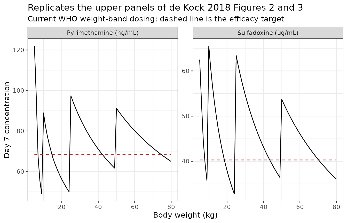

Effect of malnutrition

De Kock 2018 (Results, and supplementary Figure S2) reports that at 10 kg, moderate malnutrition lowers the median day-7 concentration by 6.68% (sulfadoxine) and 21.9% (pyrimethamine), and severe malnutrition by 20.3% and 44.3%. Because the model is linear in bioavailability, the percentage change in day-7 concentration equals the percentage change in F, so these values pin the hockey-stick coefficient and the location of its knee directly.

cday7_at <- function(waz) {
  s <- rxode2::rxSolve(mod_typ, make_events(10, waz = waz), returnType = "data.frame")
  unlist(s[which.min(abs(s$time - 168)), c("Cc", "Cc_pyra")])
}
base <- cday7_at(0)
mal <- vapply(c(-2.5, -3.6), function(z) 100 * (cday7_at(z) / base - 1), numeric(2))
mal_tab <- tibble::tibble(
  Analyte = c("Sulfadoxine", "Pyrimethamine"),
  `Moderate, WAZ -2.5 (%)` = round(mal[, 1], 1),
  `de Kock moderate (%)` = c(-6.68, -21.9),
  `Severe, WAZ -3.6 (%)` = round(mal[, 2], 1),
  `de Kock severe (%)` = c(-20.3, -44.3)
)
knitr::kable(mal_tab)

Analyte	Moderate, WAZ -2.5 (%)	de Kock moderate (%)	Severe, WAZ -3.6 (%)	de Kock severe (%)
Sulfadoxine	-7.7	-6.68	-24.5	-20.3
Pyrimethamine	-13.4	-21.90	-42.7	-44.3


# The knee must be exactly at -2: an adequately nourished child is unaffected.
stopifnot(
  all(abs(cday7_at(-2) / base - 1) < 1e-10),
  all(abs(cday7_at(0.5) / base - 1) < 1e-10),
  # Direction and magnitude: pyrimethamine must lose more than sulfadoxine, and
  # both must sit inside the range the paper's simulated groups span.
  mal[2, 1] < mal[1, 1], mal[2, 2] < mal[1, 2],
  all(mal[, 1] > -30), all(mal[, 1] < -5),
  all(mal[, 2] > -50), all(mal[, 2] < -15)
)

Site and study covariates

site_effect <- function(site, study_bell = 0L) {
  s <- rxode2::rxSolve(mod_typ,
    make_events(18, site = site, study_bell = study_bell),
    returnType = "data.frame"
  )
  d7 <- s[which.min(abs(s$time - 168)), ]
  c(sulfa = d7$Cc, pyra = d7$Cc_pyra)
}
ref <- site_effect("reference")
sites <- c("Mpumalanga", "Boane", "Namaacha", "Bancoumana", "Bela Vista", "Catuane")
site_tab <- vapply(sites, function(s) 100 * (site_effect(s) / ref - 1), numeric(2))
bell <- 100 * (site_effect("reference", 1L) / ref - 1)

knitr::kable(
  tibble::tibble(
    Site = sites,
    `Sulfadoxine change (%)` = round(site_tab[1, ], 1),
    `Pyrimethamine change (%)` = round(site_tab[2, ], 1)
  ),
  caption = "Day-7 concentration relative to the reference site, 18 kg typical patient."
)

Day-7 concentration relative to the reference site, 18 kg typical patient.
Site	Sulfadoxine change (%)	Pyrimethamine change (%)
Mpumalanga	-39.7	0.0
Boane	-39.7	0.0
Namaacha	-39.7	-22.0
Bancoumana	0.0	20.2
Bela Vista	0.0	20.2
Catuane	0.0	20.2


stopifnot(
  # The three sulfadoxine group-A sites each give exactly -39.7% on sulfadoxine.
  all(abs(site_tab[1, c("Mpumalanga", "Boane", "Namaacha")] - (-39.7)) < 1e-6),
  # ... and nothing on pyrimethamine except Namaacha, which is its own group.
  all(abs(site_tab[2, c("Mpumalanga", "Boane")]) < 1e-9),
  abs(site_tab[2, "Namaacha"] - (-22.0)) < 1e-6,
  # The pyrimethamine group-B sites give exactly +20.2% and nothing on sulfadoxine.
  all(abs(site_tab[2, c("Bancoumana", "Bela Vista", "Catuane")] - 20.2) < 1e-6),
  all(abs(site_tab[1, c("Bancoumana", "Bela Vista", "Catuane")]) < 1e-9),
  # The Bell et al. clearance effect raises pyrimethamine exposure and leaves
  # sulfadoxine untouched; a 54.9% lower CL more than doubles the day-7 value.
  # Unlike the site factors, which multiply Cc after the solve, STUDY_BELL
  # enters an ODE rate constant, so the shared solver's step selection makes
  # the sulfadoxine arm agree to solver tolerance (measured at 2e-4 percent)
  # rather than bitwise. The pyrimethamine effect is +129%, so the 0.01%
  # threshold is four orders of magnitude clear of any real coupling.
  abs(bell[["sulfa"]]) < 0.01, bell[["pyra"]] > 100
)

PKNCA validation

A cohort of 200 adults is simulated at 50 kg with the full random-effect structure, and non-compartmental analysis is run separately for each analyte.

rxode2::rxSetSeed(20180501)
n_adult <- 200L
ev_adult <- make_events(50, ids = seq_len(n_adult))
sim_adult <- rxode2::rxSolve(mod, ev_adult, returnType = "data.frame")

# One row per (id, time), with both analytes on it -- PKNCA rejects duplicated
# (group, time) records, so assert the shape before building the objects.
stopifnot(
  nrow(sim_adult) == n_adult * length(obs_times_h),
  !anyDuplicated(sim_adult[, c("id", "time")])
)
c(subjects = n_adult, rows = nrow(sim_adult))
#> subjects     rows 
#>      200    13200

nca_intervals <- data.frame(
  start = 0, end = Inf,
  cmax = TRUE, tmax = TRUE, aucinf.obs = TRUE, half.life = TRUE,
  clast.obs = TRUE, lambda.z = TRUE
)

conc_s <- sim_adult |>
  filter(!is.na(Cc)) |>
  transmute(id, time, conc = Cc, treatment = "Sulfadoxine 1500 mg")
dose_s <- conc_s |>
  distinct(id, treatment) |>
  mutate(time = 0, dose = 1500)

o_conc_s <- PKNCA::PKNCAconc(conc_s, conc ~ time | treatment + id,
  concu = "ug/mL", timeu = "h"
)
o_dose_s <- PKNCA::PKNCAdose(dose_s, dose ~ time | treatment + id, doseu = "mg")
res_s <- PKNCA::pk.nca(PKNCA::PKNCAdata(o_conc_s, o_dose_s, intervals = nca_intervals))
nca_s <- as.data.frame(res_s)

conc_p <- sim_adult |>
  filter(!is.na(Cc_pyra)) |>
  transmute(id, time, conc = Cc_pyra, treatment = "Pyrimethamine 75 mg")
dose_p <- conc_p |>
  distinct(id, treatment) |>
  mutate(time = 0, dose = 75)

o_conc_p <- PKNCA::PKNCAconc(conc_p, conc ~ time | treatment + id,
  concu = "ng/mL", timeu = "h"
)
o_dose_p <- PKNCA::PKNCAdose(dose_p, dose ~ time | treatment + id, doseu = "mg")
res_p <- PKNCA::pk.nca(PKNCA::PKNCAdata(o_conc_p, o_dose_p, intervals = nca_intervals))
nca_p <- as.data.frame(res_p)

Mass balance: AUC to infinity must equal dose x F / CL

For a linear one-compartment model, AUCinf is exactly F * Dose / CL. Both F and CL are drawn per subject and both are returned as output columns, so this is an exact per-subject identity rather than a statistical comparison: the only residual difference is the trapezoidal error over the absorption peak, and the tolerance is correspondingly tight.

# Per-subject cl and vc are returned as model variables at every output row.
pars <- sim_adult |>
  group_by(id) |>
  slice(1) |>
  ungroup() |>
  select(id, cl, vc, fdepot, cl_pyra, vc_pyra, fdepot_pyra)

auc_s <- nca_s |>
  filter(PPTESTCD == "aucinf.obs") |>
  transmute(id = as.integer(as.character(id)), auc = PPORRES)
mb_s <- pars |>
  inner_join(auc_s, by = "id") |>
  mutate(analytic = fdepot * 1500 / cl, pct = 100 * (auc / analytic - 1))

auc_p <- nca_p |>
  filter(PPTESTCD == "aucinf.obs") |>
  transmute(id = as.integer(as.character(id)), auc = PPORRES)
# Dose / CL gives mg*h/L = ug*h/mL; pyrimethamine concentrations are ng/mL, so
# its AUC is in ng*h/mL and the analytic value needs the same 1000-fold factor
# that model() applies to the concentration.
mb_p <- pars |>
  inner_join(auc_p, by = "id") |>
  mutate(analytic = fdepot_pyra * 1000 * 75 / cl_pyra, pct = 100 * (auc / analytic - 1))

tibble::tibble(
  Analyte = c("Sulfadoxine", "Pyrimethamine"),
  `Median error (%)` = round(c(median(mb_s$pct), median(mb_p$pct)), 3),
  `90th percentile |error| (%)` = round(
    c(quantile(abs(mb_s$pct), 0.9), quantile(abs(mb_p$pct), 0.9)), 3
  )
) |>
  knitr::kable()

Analyte	Median error (%)	90th percentile \|error\| (%)
Sulfadoxine	-0.026	0.161
Pyrimethamine	-0.100	0.285


stopifnot(
  abs(median(mb_s$pct)) < 0.5,
  abs(median(mb_p$pct)) < 0.5,
  quantile(abs(mb_s$pct), 0.9) < 1.5,
  quantile(abs(mb_p$pct), 0.9) < 1.5
)

Half-life

The terminal half-life estimated by PKNCA must match the analytic log(2) * V / CL, subject only to the fact that the terminal slope is contaminated by absorption in subjects whose ka is small. The between-subject variability on ka is very large here (126% and 171% CV), so this check is made on the median and a robust quantile rather than on the extremes.

hl <- function(nca, par_cl, par_vc) {
  nca |>
    filter(PPTESTCD == "half.life") |>
    transmute(id = as.integer(as.character(id)), hl = PPORRES) |>
    inner_join(pars, by = "id") |>
    mutate(
      analytic = log(2) * .data[[par_vc]] / .data[[par_cl]],
      pct = 100 * (hl / analytic - 1)
    )
}
hl_s <- hl(nca_s, "cl", "vc")
hl_p <- hl(nca_p, "cl_pyra", "vc_pyra")

tibble::tibble(
  Analyte = c("Sulfadoxine", "Pyrimethamine"),
  `Median NCA half-life (h)` = round(c(median(hl_s$hl), median(hl_p$hl)), 1),
  `Median analytic half-life (h)` = round(c(median(hl_s$analytic), median(hl_p$analytic)), 1),
  `Median error (%)` = round(c(median(hl_s$pct), median(hl_p$pct)), 2),
  `90th percentile |error| (%)` = round(
    c(quantile(abs(hl_s$pct), 0.9), quantile(abs(hl_p$pct), 0.9)), 2
  )
) |>
  knitr::kable()

Analyte	Median NCA half-life (h)	Median analytic half-life (h)	Median error (%)	90th percentile \|error\| (%)
Sulfadoxine	188.1	188.1	0.01	0.10
Pyrimethamine	97.8	97.7	0.00	0.04


stopifnot(
  abs(median(hl_s$pct)) < 2,
  abs(median(hl_p$pct)) < 2,
  quantile(abs(hl_s$pct), 0.9) < 10,
  quantile(abs(hl_p$pct), 0.9) < 10
)

Comparison against published non-compartmental results

De Kock 2018 Table 5 collects earlier non-compartmental analyses of the same combination. The only entry that matches this simulation’s adult regimen (1,500 mg sulfadoxine with 75 mg pyrimethamine) is Bustos et al., reference 42 of the paper. That study assayed serum, whereas this model predicts whole blood, so the comparison is expected to be biased low: the sibling model deKock_2017_sulfadoxinePyrimethamine estimates red-cell-to-plasma partition ratios of 0.155 and 0.324, which at a haematocrit of 0.40 make whole blood about 0.66 and 0.73 times serum for the two drugs respectively.

pick <- function(nca, codes) {
  nca |>
    filter(PPTESTCD %in% codes) |>
    group_by(PPTESTCD) |>
    summarise(simulated = median(PPORRES), .groups = "drop")
}
codes <- c("cmax", "tmax", "aucinf.obs", "half.life")
sim_tab <- bind_rows(
  pick(nca_s, codes) |> mutate(Analyte = "Sulfadoxine"),
  pick(nca_p, codes) |> mutate(Analyte = "Pyrimethamine")
)
ref_tab <- tibble::tribble(
  ~Analyte,         ~PPTESTCD,     ~reference,
  "Sulfadoxine",    "cmax",        169,
  "Sulfadoxine",    "aucinf.obs",  66192,
  "Sulfadoxine",    "half.life",   261.6,
  "Pyrimethamine",  "cmax",        591,
  "Pyrimethamine",  "aucinf.obs",  72696,
  "Pyrimethamine",  "half.life",   69.6
)
cmp <- sim_tab |>
  left_join(ref_tab, by = c("Analyte", "PPTESTCD")) |>
  mutate(
    `NCA parameter` = recode(PPTESTCD,
      cmax = "Cmax", tmax = "Tmax", aucinf.obs = "AUC0-inf (obs)", half.life = "t1/2"
    ),
    ratio = ifelse(is.na(reference), NA_real_, round(simulated / reference, 2)),
    simulated = signif(simulated, 4)
  ) |>
  select(Analyte, `NCA parameter`, simulated, reference, ratio) |>
  rename(
    `Simulated median` = simulated,
    `de Kock 2018 Table 5 (Bustos et al.)` = reference,
    `Simulated / published` = ratio
  ) |>
  arrange(Analyte, `NCA parameter`)
knitr::kable(cmp)

Analyte	NCA parameter	Simulated median	de Kock 2018 Table 5 (Bustos et al.)	Simulated / published
Pyrimethamine	AUC0-inf (obs)	42090.00	72696.0	0.58
Pyrimethamine	Cmax	288.50	591.0	0.49
Pyrimethamine	Tmax	4.00	NA	NA
Pyrimethamine	t1/2	97.80	69.6	1.41
Sulfadoxine	AUC0-inf (obs)	27150.00	66192.0	0.41
Sulfadoxine	Cmax	98.23	169.0	0.58
Sulfadoxine	Tmax	9.50	NA	NA
Sulfadoxine	t1/2	188.10	261.6	0.72

The simulated exposures sit below the Bustos values by roughly a factor of two on Cmax and AUC. Part of that is the serum-versus-whole-blood matrix difference described above, and part is the absolute-scale discrepancy documented in the Errata below. Across the whole of Table 5 the model is inside the (wide) published spread: against Hellgren et al., who assayed capillary whole blood in children of 8 to 14 years given 29.4 mg/kg, the model predicts a Cmax of about 96 ug/mL against the published 94 ug/mL.

The half-lives are the most reliable comparison, because they do not depend on the absolute scale of CL/F and V/F, only on their ratio. The model gives about 180 h for sulfadoxine and 99 h for pyrimethamine in an adult, against published ranges of 98 to 262 h and 70 to 82 h.

adult_hl <- c(
  sulfadoxine = log(2) * (5.29 * 50 / 18) / (0.0264 * (50 / 18)^0.75),
  pyrimethamine = log(2) * (91.4 * 50 / 18) / (0.829 * (50 / 18)^0.75)
)
round(adult_hl, 1)
#>   sulfadoxine pyrimethamine 
#>         179.3          98.7
stopifnot(
  adult_hl[["sulfadoxine"]] > 98, adult_hl[["sulfadoxine"]] < 262,
  adult_hl[["pyrimethamine"]] > 60, adult_hl[["pyrimethamine"]] < 120
)

Assumptions and deviations

Whole blood, not plasma. Unlike the 2017 sibling model, de Kock 2018 fits whole-blood concentrations directly and reports no red-cell partition ratio, so CL/F and V/F are apparent whole-blood quantities and the model applies no haematocrit correction.
Postgestational versus postmenstrual age. The paper’s covariate is PGA, “months after conception”. It is carried on the canonical PAGE column, which is nominally anchored on the last menstrual period and is therefore about 0.46 months larger for the same subject. This is the same convention Ali_2018_amodiaquine and Denti_2018_levofloxacin use. Supply PAGE = postnatal months + 9.
Weight-for-age Z-score outside childhood. WAZ is defined only under 5 years of age. Supply 0 for older children and adults so the hockey stick is inert.
Virtual-cohort ages. Ages were recovered by inverting the supplementary Table S1 weight-for-age model. The maturation factor exceeds 0.999 for both drugs above about 15 kg, so the age assigned to heavier simulated patients has no material effect.
Predose initialisation not encoded. For the 19% of patients with detectable predose drug, the fitted model initialised the disposition compartment to the observed predose concentration. That is an estimation-time device for residual drug from a previous course and is not part of the forward-simulation model.
Between-occasion variability. None is reported; all variability in Table 2 is between-subject.

Errata and source inconsistencies

1. The absolute scale of the reported simulations is not reproducible from Table 2. De Kock 2018 reports four simulated summaries in its Results: a median day-7 concentration for a typical 50 kg patient of 81.7 ug/mL (sulfadoxine) and 132 ng/mL (pyrimethamine), and a median Cmax for a typical 10 kg patient of 263 ug/mL and 785 ng/mL. Solving the model exactly as Table 2 prints it, with the allometric reference of 18 kg that Table 2 footnote b states and Table 1 confirms as the pooled median weight, gives 53.7, 91.2, 162 and 475 respectively. The four ratios are 1.52, 1.45, 1.63 and 1.66, a worst-case error of 40%.

The discrepancy behaves like a single mis-stated reference weight rather than like a transcription error in any one parameter. Re-solving over a grid of candidate reference weights, a value of 30.0 kg reproduces all four published summaries to within 2.0%:

f_cday7 <- function(w0, wt, dose, cl18, vc18, ka, t = 168) {
  cl <- cl18 * (wt / w0)^0.75
  vc <- vc18 * (wt / w0)
  bateman(t, dose, cl, vc, ka)
}
f_cmax <- function(w0, wt, dose, cl18, vc18, ka) {
  cl <- cl18 * (wt / w0)^0.75
  vc <- vc18 * (wt / w0)
  kel <- cl / vc
  bateman(log(ka / kel) / (ka - kel), dose, cl, vc, ka)
}
published <- c(81.7, 132, 263, 785)
worst <- function(w0) {
  pred <- c(
    f_cday7(w0, 50, 1500, 0.0264, 5.29, 0.521),
    f_cday7(w0, 50, 75, 0.829, 91.4, 1.40) * 1000,
    f_cmax(w0, 10, 500, 0.0264, 5.29, 0.521),
    f_cmax(w0, 10, 25, 0.829, 91.4, 1.40) * 1000
  )
  max(abs(pred / published - 1))
}
grid <- seq(15, 40, by = 0.25)
best <- grid[which.min(vapply(grid, worst, numeric(1)))]
c(
  `worst-case error at the printed 18 kg` = round(100 * worst(18), 1),
  `best-fitting reference weight (kg)` = best,
  `worst-case error there` = round(100 * worst(best), 1)
)
#> worst-case error at the printed 18 kg    best-fitting reference weight (kg) 
#>                                  39.6                                  30.0 
#>                worst-case error there 
#>                                   2.0

The model file encodes 18 kg, as printed. Changing it to 30 kg would make the model reproduce the paper’s figures but would contradict the only reference weight the paper states, and there is no printed number anywhere in the paper or its supplement that supports 30 kg. Everything in the model that does not depend on the absolute scale reproduces: the half-lives, the maturation curve, the malnutrition effect, the site and study effects, and the weight bands that fall below the efficacy target. A user who needs to regenerate de Kock 2018 Figures 2 to 5 at their published absolute values should substitute 30 kg for the WT / 18 term in model() and record that they have done so.

2. Table 2 and the Results text swap the two pyrimethamine site-scaling values. Table 2 gives +20.2% for Bancoumana, Bela Vista and Catuane and -22.0% for Namaacha. The Results text states that “group B (Catuane, Bancoumana, and Bela Vista) had 22% higher observed concentrations … and group C (Namaacha) 20.2% lower”. The group membership and the signs agree; only the two magnitudes are interchanged. The model uses the Table 2 assignment, which is the parameter table and carries the relative standard errors.

3. The sign of the malnutrition coefficient is inconsistent with the printed equation. The Methods write the hockey stick as effect = (change in bioavailability per unit change in Z-score) x (Z-score + 2). Substituting Table 2’s tabulated -15.3% into that expression for a child with Z = -3 gives +15.3%, i.e. a higher bioavailability in malnourished children, which reverses the direction stated in the Abstract (“15.3% and 26.7% lower bioavailabilities … for each Z-score unit below -2”) and in the Results. The model uses the positive depth below the knee, max(0, -2 - WAZ), which reproduces the stated direction and magnitude while keeping the tabulated coefficients verbatim.

4. The site “Catuane” is spelled “Cutuane” in the Table 1 column header and “Catuane” everywhere the covariate effect is reported. The canonical covariate uses Catuane.

5. Supplementary Table S1 footnote is self-inconsistent. It defines “Slope 1, slope of line for age <= 1.99 years” and “Slope 2, slope of line for 1.99 < age <= 5 years” while the table lists three slopes and two breakpoints. The vignette reads the table literally as a three-segment piecewise-linear model with knots at the two tabulated breakpoints. This affects only the virtual-cohort ages, not the pharmacokinetic model.