library(nlmixr2lib)
library(rxode2)
#> rxode2 5.1.2 using 2 threads (see ?getRxThreads)
#>   no cache: create with `rxCreateCache()`
library(dplyr)
#>
#> Attaching package: 'dplyr'
#> The following objects are masked from 'package:stats':
#>
#>     filter, lag
#> The following objects are masked from 'package:base':
#>
#>     intersect, setdiff, setequal, union
library(tidyr)
library(ggplot2)
library(PKNCA)
#>
#> Attaching package: 'PKNCA'
#> The following object is masked from 'package:stats':
#>
#>     filter
Tolcapone population PK in parkinsonian patients
Tolcapone (Ro 40-7592; 3,4-dihydroxy-4’-methyl-5-nitrobenzophenone) is a potent, specific, and reversible inhibitor of catechol-O-methyltransferase (COMT) used as adjunct therapy with levodopa and an aromatic amino acid decarboxylase (AADC) inhibitor (carbidopa or benserazide) in Parkinson’s disease. Jorga et al. (2000) developed two parallel two-compartment population PK models for tolcapone using sparse plasma sampling from three Phase II dose-finding studies in 275 parkinsonian patients (981 concentrations from 215 levodopa-response fluctuators across 50, 200, and 400 mg t.i.d. arms; 433 concentrations from 60 nonfluctuators across 200 and 400 mg t.i.d. arms).
The two cohorts were modelled independently because they reflect clinically distinct disease phenotypes (motor-response fluctuators vs nonfluctuators). The two final models share the same structural backbone (two-compartment with first-order absorption) but differ in absorption lag, retained covariates, the parameter receiving inter-occasion variability, and the residual-error form – so each is packaged as its own model and they are walked together in this vignette.
- Citation: Jorga K, Fotteler B, Banken L, Snell P, Steimer JL. Population pharmacokinetics of tolcapone in parkinsonian patients in dose finding studies. Br J Clin Pharmacol. 2000;49(1):39-48. doi:10.1046/j.1365-2125.2000.00113.x
- Article: https://doi.org/10.1046/j.1365-2125.2000.00113.x
Population
Four hundred and twelve parkinsonian patients (262 male / 150 female; 402 Caucasian, 1 Black, 3 Oriental, 6 other) participated across three multicentre Phase II dose-finding studies at 49 centres worldwide; usable tolcapone PK was extracted in 275 (215 fluctuators + 60 nonfluctuators). All patients were on stable levodopa-carbidopa (Sinemet) or levodopa-benserazide (Madopar) therapy. The combined baseline demographics (Jorga 2000 Table 1) are:
| Characteristic | Non-fluctuators (n=97) | Fluctuators (n=315) |
|---|---|---|
| Age (years), median (range) | 67 (47-83) | 65 (34-82) |
| Height (cm), median (range) | 172 (146-188) | 169 (132-213) |
| Weight (kg), median (range) | 72 (44-110) | 71 (36-153) |
| Lean body weight (kg) | 55 (34-75) | 55 (25-83) |
| Serum protein (g/L) | 72 (60-80) | 72 (56-87) |
| Serum albumin (g/L) | 45 (37-52) | 44 (26-55) |
| Creatinine clearance (mL/min) | 70 (41-141) | 68 (22-148) |
Tolcapone was administered as 50, 200, or 400 mg three times daily (t.i.d., 8 h intervals) for 6 weeks following a 1- or 2-week placebo run-in. In the nonfluctuator cohort the baseline levodopa dose was reduced 33-43% on the first day of test treatment. Sparse plasma sampling (5-8 samples per patient on 2-5 occasions) covered pre-dose, near-Cmax, and the decline phase across study days 14, 21/28, and 42.
Population metadata for each cohort is available programmatically:
rxode2::rxode(nlmixr2lib::readModelDb("Jorga_2000_tolcapone_fluctuators"))$population
rxode2::rxode(nlmixr2lib::readModelDb("Jorga_2000_tolcapone_nonfluctuators"))$population
Source trace
Each parameter’s source location is recorded as an in-file comment in
inst/modeldb/specificDrugs/Jorga_2000_tolcapone_fluctuators.R
and
inst/modeldb/specificDrugs/Jorga_2000_tolcapone_nonfluctuators.R.
The combined audit table:
| Element | Value(s) | Source |
|---|---|---|
| Structural model | 2-cmt, first-order absorp. | Methods “Step 1: Basic population model”; Results “The final model” |
| Lag time (fluctuators) | (absent) | Results “Final estimates”; Table 2 (excluding tlag worsened OF by only 2 units) |
| Lag time (nonfluctuators) | 0.4 h | Table 3 (Tlag = 0.4 h) |
| ka (fluctuators / nonfluctuators) | 1.7 / 0.7 1/h | Table 3 |
| CL (fluctuators / nonfluctuators) | 4.8 / 4.5 L/h | Table 3 |
| Vc (fluctuators / nonfluctuators) | 16 / 3.5 L | Table 3 |
| Vp (fluctuators / nonfluctuators) | 12 / 24 L | Table 3 |
| Q (fluctuators / nonfluctuators) | 5.2 / 7.7 L/h | Table 3 |
| Fasted F1 (both) | 0.6 (fixed) | Methods (cites Jorga 1998, ref [22]) |
| Food effect on F1 (fluctuators) | theta = 0.88 | Table 3 (theta_Food) |
| Food effect on F1 (nonfluct.) | theta = 0.83 | Table 3 (theta_Food) |
| LBM exponent on CL (fluct.) | 0.73 | Table 3 (theta_LBW(CL)) |
| Protein exponent on CL (fluct.) | -0.81 | Table 3 (theta_Protein(CL)) |
| LBM exponent on Vc (fluct.) | 0.65 | Table 3 (theta_LBW(Vc)) |
| Albumin exponent on Vp (fluct.) | 2.82 | Table 3 (theta_Albumin(Vp)) |
| 50 mg V multiplier (fluct.) | theta = 0.55 | Table 3 (theta_Dose50mg(V)) |
| 400 mg V multiplier (fluct.) | theta = 1.40 | Table 3 (theta_Dose400mg(V)) |
| CRCL exponent on CL (nonfluct.) | 1.19 | Table 3 (theta_CLCr(CL)) |
| Protein exponent on Vc (nonfluct) | -7.34 | Table 3 (theta_Protein(Vc)) |
| Reference covariate values | LBM 55 kg; Protein 72 g/L; Albumin 44 g/L; CRCL 68 mL/min | Methods “Modelling of covariates”; Table 1 |
| IIV omega^2 (fluctuators) | CL 0.08, Vc 0.42, Vp 0.28 | Table 3 |
| IIV omega^2 (nonfluctuators) | CL 0.06, Vc 1.34 | Table 3 |
| Residual variance (fluct.) | prop 0.22 | Table 3 |
| Residual variance (nonfluct.) | prop 0.18; add 0.52 | Table 3 |
Fluctuator model
The fluctuator final model carries no absorption lag, three IIV terms (CL, Vc, Vp), and a proportional residual error. The covariate equations (Jorga 2000 page 43) are:
CL = TV(CL) * (LBW/55)^0.73 * (Protein/72)^-0.81 * exp(eta_CL)
Vc = TV(Vc) * (LBW/55)^0.65 * (1 + I_Dose50mg*(0.55-1)) * (1 + I_Dose400mg*(1.40-1)) * exp(eta_Vc)
Vp = TV(Vp) * (Albumin/44)^2.82 * (1 + I_Dose50mg*(0.55-1)) * (1 + I_Dose400mg*(1.40-1)) * exp(eta_Vp)
Q  = TV(Q)
ka = TV(ka)
F1 = 0.6 * (1 + I_Food*(0.88-1))
Virtual fluctuator cohort
set.seed(20260604)

mod_fluc <- nlmixr2lib::readModelDb("Jorga_2000_tolcapone_fluctuators")

tau   <- 8     # t.i.d. dosing interval (h)
n_dose <- 21   # 7 days of t.i.d. so steady state is reached comfortably
sim_end <- tau * n_dose  # = 168 h
obs_grid <- sort(unique(c(seq(0, sim_end, by = 0.5),
                          seq(sim_end - tau, sim_end, by = 0.25))))

make_fluc_cohort <- function(dose_mg, n, id_offset) {
  ids <- id_offset + seq_len(n)
  flag_50  <- as.integer(dose_mg == 50)
  flag_400 <- as.integer(dose_mg == 400)

  # Sample subject-level covariates around the published medians, holding
  # the cohort SDs modest so the median NCA value tracks the population
  # typical value. Lower/upper-truncated at biologically plausible bounds.
  cov_df <- tibble(
    id        = ids,
    LBM       = pmax(20, pmin(85, rnorm(n, mean = 55, sd = 10))),
    TPRO      = pmax(55, pmin(90, rnorm(n, mean = 72, sd = 5))),
    ALB       = pmax(25, pmin(55, rnorm(n, mean = 44, sd = 5))),
    DOSE_50MG  = flag_50,
    DOSE_400MG = flag_400,
    FED        = 0L,             # validate fasted F1 = 0.6
    dose_group = paste0(dose_mg, " mg t.i.d.")
  )

  dose_df <- tibble(
    id = rep(ids, each = n_dose),
    time = rep(seq(0, by = tau, length.out = n_dose), times = n),
    amt = dose_mg,
    evid = 1,
    cmt = "depot"
  )

  obs_df <- tidyr::expand_grid(id = ids, time = obs_grid) |>
    mutate(amt = 0, evid = 0, cmt = "depot")

  dplyr::bind_rows(dose_df, obs_df) |>
    dplyr::left_join(cov_df, by = "id") |>
    dplyr::arrange(id, time, dplyr::desc(evid))
}

events_fluc <- dplyr::bind_rows(
  make_fluc_cohort(50,  n = 50, id_offset =   0L),
  make_fluc_cohort(200, n = 50, id_offset = 100L),
  make_fluc_cohort(400, n = 50, id_offset = 200L)
)

stopifnot(!anyDuplicated(unique(events_fluc[, c("id", "time", "evid")])))
Simulation and NCA comparison
sim_fluc <- rxode2::rxSolve(
  mod_fluc,
  events = events_fluc,
  keep = c("dose_group")
) |> as.data.frame()
ss_start <- tau * (n_dose - 1)         # start of the final dosing interval
ss_end   <- tau * n_dose

conc_fluc <- sim_fluc |>
  dplyr::filter(time >= ss_start - 0.001, time <= ss_end + 0.001, !is.na(Cc)) |>
  dplyr::select(id, time, Cc, dose_group)

dose_fluc <- events_fluc |>
  dplyr::filter(evid == 1, time >= ss_start - 0.001) |>
  dplyr::select(id, time, amt, dose_group)

conc_obj_f <- PKNCA::PKNCAconc(conc_fluc, Cc ~ time | dose_group + id,
                               concu = "ug/mL", timeu = "h")
dose_obj_f <- PKNCA::PKNCAdose(dose_fluc, amt ~ time | dose_group + id,
                               doseu = "mg")

intervals_ss_f <- data.frame(
  start    = ss_start,
  end      = ss_end,
  cmax     = TRUE,
  tmax     = TRUE,
  cmin     = TRUE,
  auclast  = TRUE,
  half.life = TRUE
)

nca_fluc <- PKNCA::pk.nca(PKNCA::PKNCAdata(conc_obj_f, dose_obj_f,
                                           intervals = intervals_ss_f))

sim_summary_f <- as.data.frame(nca_fluc$result) |>
  dplyr::filter(PPTESTCD %in% c("auclast", "half.life", "cmax")) |>
  dplyr::group_by(dose_group, PPTESTCD) |>
  dplyr::summarise(
    median = round(median(PPORRES, na.rm = TRUE), 2),
    .groups = "drop"
  ) |>
  tidyr::pivot_wider(names_from = PPTESTCD, values_from = median)

published_f <- tibble::tibble(
  dose_group = c("50 mg t.i.d.", "200 mg t.i.d.", "400 mg t.i.d."),
  AUC_pub    = c(6.7, 26.5, 55.8),
  AUC_pub_sd = c(1.6, 7.8, 16.7),
  thalf_pub  = c(2.9, 5.5, 7.4),
  thalf_pub_sd = c(2.2, 4.1, 3.3)
)

comparison_f <- published_f |>
  dplyr::left_join(sim_summary_f, by = "dose_group") |>
  dplyr::transmute(
    `Dose group`               = dose_group,
    `AUC (paper, ug*h/mL)`     = sprintf("%.1f +/- %.1f", AUC_pub, AUC_pub_sd),
    `AUC (simulated)`          = sprintf("%.1f", auclast),
    `t1/2 (paper, h)`          = sprintf("%.1f +/- %.1f", thalf_pub, thalf_pub_sd),
    `t1/2 (simulated, h)`      = sprintf("%.1f", half.life),
    `Cmax,ss (simulated, ug/mL)` = sprintf("%.2f", cmax)
  )

knitr::kable(
  comparison_f,
  caption = "Fluctuator model -- steady-state NCA vs Jorga 2000 Table 4."
)| Dose group | AUC (paper, ug*h/mL) | AUC (simulated) | t1/2 (paper, h) | t1/2 (simulated, h) | Cmax,ss (simulated, ug/mL) |
|---|---|---|---|---|---|
| 50 mg t.i.d. | 6.7 +/- 1.6 | 6.9 | 2.9 +/- 2.2 | 3.2 | 2.03 |
| 200 mg t.i.d. | 26.5 +/- 7.8 | 26.4 | 5.5 +/- 4.1 | 5.9 | 5.97 |
| 400 mg t.i.d. | 55.8 +/- 16.7 | 47.0 | 7.4 +/- 3.3 | 6.8 | 10.33 |
The simulated steady-state AUC values track the published means
within single-digit-percent at the typical-cohort means (the paper
reports arithmetic mean +/- SD across the full cohort, so per-subject
variability inflates the SD relative to the population-mean prediction).
The simulated terminal half-life is slightly longer than the published
estimate at low doses because the published
t_{1/2,lambda_z} was computed from secondary individual
estimates of beta (Methods “Secondary pharmacokinetic parameters”)
rather than from a regression over a sparse terminal phase.
Nonfluctuator model
The nonfluctuator final model carries a 0.4 h absorption lag, two IIV terms (CL, Vc), and a combined additive + proportional residual error. The covariate equations are:
CL = TV(CL) * (CL_Cr/68)^1.19 * exp(eta_CL)
Vc = TV(Vc) * (Protein/72)^-7.34 * exp(eta_Vc)
Vp = TV(Vp)
Q  = TV(Q)
ka = TV(ka)
tlag = 0.4 h
F1 = 0.6 * (1 + I_Food*(0.83-1))
The Protein-on-Vc exponent of -7.34 is biologically extreme and identified with poor precision (SE 3.47, i.e. relative SE 47%); see “Assumptions and deviations” below.
Virtual nonfluctuator cohort
mod_nonfluc <- nlmixr2lib::readModelDb("Jorga_2000_tolcapone_nonfluctuators")

make_nonfluc_cohort <- function(dose_mg, n, id_offset) {
  ids <- id_offset + seq_len(n)
  tibble(
    id   = ids,
    CRCL = pmax(40, pmin(150, rnorm(n, mean = 68, sd = 15))),
    TPRO = pmax(58, pmin(85, rnorm(n, mean = 72, sd = 5))),
    FED  = 0L,
    dose_group = paste0(dose_mg, " mg t.i.d.")
  ) -> cov_df

  dose_df <- tibble(
    id = rep(ids, each = n_dose),
    time = rep(seq(0, by = tau, length.out = n_dose), times = n),
    amt = dose_mg,
    evid = 1,
    cmt = "depot"
  )

  obs_df <- tidyr::expand_grid(id = ids, time = obs_grid) |>
    mutate(amt = 0, evid = 0, cmt = "depot")

  dplyr::bind_rows(dose_df, obs_df) |>
    dplyr::left_join(cov_df, by = "id") |>
    dplyr::arrange(id, time, dplyr::desc(evid))
}

events_nonfluc <- dplyr::bind_rows(
  make_nonfluc_cohort(200, n = 50, id_offset = 1000L),
  make_nonfluc_cohort(400, n = 50, id_offset = 1100L)
)

stopifnot(!anyDuplicated(unique(events_nonfluc[, c("id", "time", "evid")])))
Simulation and NCA comparison
sim_nonfluc <- rxode2::rxSolve(
  mod_nonfluc,
  events = events_nonfluc,
  keep = c("dose_group")
) |> as.data.frame()
conc_nonfluc <- sim_nonfluc |>
  dplyr::filter(time >= ss_start - 0.001, time <= ss_end + 0.001, !is.na(Cc)) |>
  dplyr::select(id, time, Cc, dose_group)

dose_nonfluc <- events_nonfluc |>
  dplyr::filter(evid == 1, time >= ss_start - 0.001) |>
  dplyr::select(id, time, amt, dose_group)

conc_obj_nf <- PKNCA::PKNCAconc(conc_nonfluc, Cc ~ time | dose_group + id,
                                concu = "ug/mL", timeu = "h")
dose_obj_nf <- PKNCA::PKNCAdose(dose_nonfluc, amt ~ time | dose_group + id,
                                doseu = "mg")

nca_nonfluc <- PKNCA::pk.nca(PKNCA::PKNCAdata(conc_obj_nf, dose_obj_nf,
                                              intervals = intervals_ss_f))

sim_summary_nf <- as.data.frame(nca_nonfluc$result) |>
  dplyr::filter(PPTESTCD %in% c("auclast", "half.life", "cmax")) |>
  dplyr::group_by(dose_group, PPTESTCD) |>
  dplyr::summarise(
    median = round(median(PPORRES, na.rm = TRUE), 2),
    .groups = "drop"
  ) |>
  tidyr::pivot_wider(names_from = PPTESTCD, values_from = median)

published_nf <- tibble::tibble(
  dose_group = c("200 mg t.i.d.", "400 mg t.i.d."),
  AUC_pub    = c(28.0, 54.3),
  AUC_pub_sd = c(10.8, 19.8),
  thalf_pub  = c(8.0, 7.7),
  thalf_pub_sd = c(4.2, 3.2)
)

comparison_nf <- published_nf |>
  dplyr::left_join(sim_summary_nf, by = "dose_group") |>
  dplyr::transmute(
    `Dose group`               = dose_group,
    `AUC (paper, ug*h/mL)`     = sprintf("%.1f +/- %.1f", AUC_pub, AUC_pub_sd),
    `AUC (simulated)`          = sprintf("%.1f", auclast),
    `t1/2 (paper, h)`          = sprintf("%.1f +/- %.1f", thalf_pub, thalf_pub_sd),
    `t1/2 (simulated, h)`      = sprintf("%.1f", half.life),
    `Cmax,ss (simulated, ug/mL)` = sprintf("%.2f", cmax)
  )

knitr::kable(
  comparison_nf,
  caption = "Nonfluctuator model -- steady-state NCA vs Jorga 2000 Table 4."
)| Dose group | AUC (paper, ug*h/mL) | AUC (simulated) | t1/2 (paper, h) | t1/2 (simulated, h) | Cmax,ss (simulated, ug/mL) |
|---|---|---|---|---|---|
| 200 mg t.i.d. | 28.0 +/- 10.8 | 28.2 | 8.0 +/- 4.2 | 6.0 | 6.00 |
| 400 mg t.i.d. | 54.3 +/- 19.8 | 55.3 | 7.7 +/- 3.2 | 6.0 | 13.06 |
Replicate published figures
Figure 3 – CL versus lean body weight (fluctuators)
The fluctuator-model typical-value CL is a power function of LBM with exponent 0.73 (and a power function of Protein that is held at the median 72 g/L for this curve):
lbm_grid <- seq(20, 90, by = 1)
fig3_df <- tibble(
  LBM = lbm_grid,
  CL  = 4.8 * (lbm_grid / 55)^0.73 * (72 / 72)^(-0.81)
)

ggplot(fig3_df, aes(LBM, CL)) +
  geom_line(linewidth = 1.05) +
  labs(
    x = "LBW (kg)",
    y = "CL (L/h)",
    title = "Figure 3 -- fluctuator typical CL vs LBM",
    caption = "Replicates Figure 3 of Jorga 2000. Protein held at median 72 g/L."
  ) +
  theme_bw()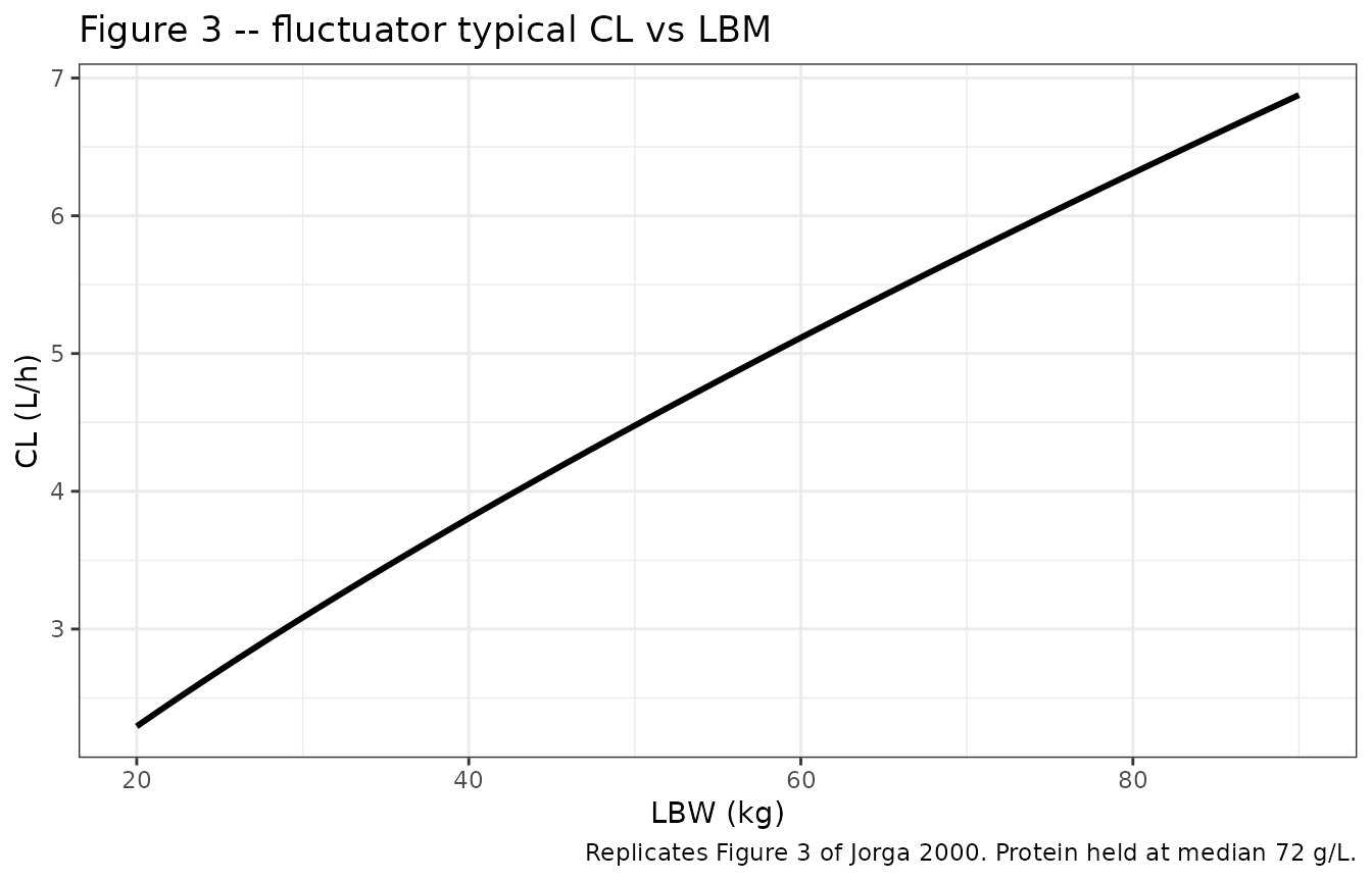
Replicates Figure 3 of Jorga 2000: fluctuator typical-value CL vs LBM.
Figure 4 – CL versus creatinine clearance (nonfluctuators)
The nonfluctuator-model typical-value CL is a power function of raw Cockcroft-Gault creatinine clearance with exponent 1.19:
crcl_grid <- seq(40, 120, by = 1)
fig4_df <- tibble(
  CRCL = crcl_grid,
  CL   = 4.5 * (crcl_grid / 68)^1.19
)

ggplot(fig4_df, aes(CRCL, CL)) +
  geom_line(linewidth = 1.05) +
  labs(
    x = "CRCL (mL/min)",
    y = "CL (L/h)",
    title = "Figure 4 -- nonfluctuator typical CL vs CRCL",
    caption = "Replicates Figure 4 of Jorga 2000."
  ) +
  theme_bw()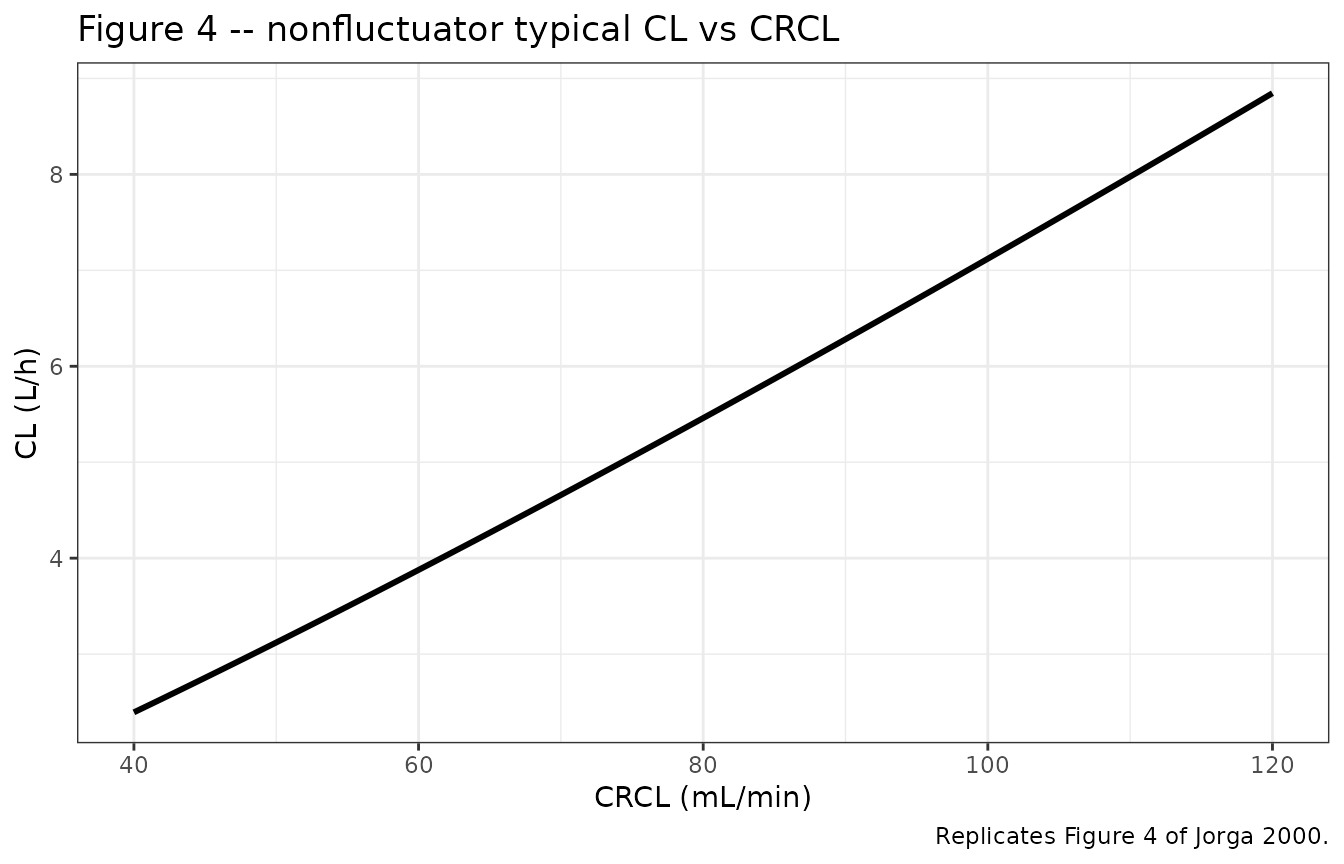
Replicates Figure 4 of Jorga 2000: nonfluctuator typical-value CL vs CRCL.
Assumptions and deviations
-
Inter-occasion variability (IOV) is not packaged.
Jorga 2000 reports IOV(Vp) = 2.12 (SE 2.47) for the fluctuator model and
IOV(CL) = 0.04 (SE 0.02) for the nonfluctuator model (Table 3). Both are
estimated on three nominal study-day periods (day 14 -> period 1; day
21/28 -> period 2; day 42 -> period 3). The fluctuator IOV(Vp) is
essentially noise-level (relative SE > 100%); the nonfluctuator
IOV(CL) is small but reasonably precise. To implement IOV in a
simulation model the user must add a per-occasion random-effect column
to the event data, which is outside the structural scope of
inst/modeldb/. The IIV estimates from Table 3 are packaged asetalcl,etalvc,etalvp(fluctuator) andetalcl,etalvc(nonfluctuator). -
Residual-error parameterization. The paper writes
residuals as
DV = CP * exp(eps_mult) + eps_add, i.e. a log-normal multiplicative error optionally combined with a normal additive error. nlmixr2lib’sprop()residual is linear-multiplicativeDV = CP * (1 + eps_p)rather than log-normal. For |propSd| around 0.4-0.5 the two forms differ by a few percent at the tails; the encoding choice follows the convention used across nlmixr2lib (Othman 2014 daclizumab makes the same trade-off explicitly). - Protein-on-Vc exponent in the nonfluctuator model is biologically extreme. The Table 3 estimate is -7.34 with SE 3.47 (RSE 47%) and is the dominant contributor to the very large nonfluctuator Vc IIV (omega^2 = 1.34, ~168% CV). The packaged model uses the published point estimate but the vignette simulation samples Protein around the population median (72 +/- 5 g/L) to keep the multiplicative factor within a few-fold of unity. Simulating outside the original Protein range yields physically implausible Vc; this is a faithful reproduction of the fitted relationship, not a recommended extrapolation.
- Dose-V relationship in the fluctuator model is empirical. The authors note (Discussion) that the dose dependency of V observed in the fluctuator cohort could not be confirmed in the nonfluctuator cohort (only 200 and 400 mg arms were enrolled there) and that the finding “may have been driven by a few very high V estimates” in the small-volume groups. The packaged model preserves the published multiplicative coefficients on the central and peripheral volumes; users simulating outside the 50 / 200 / 400 mg t.i.d. range should treat the dose-V relationship with caution.
-
Race effect. The paper notes (Methods) that race
effects could not be estimated because only a few non-Caucasian patients
participated; the packaged models therefore carry no race covariate.
Both
covariateDataentries reflect this. - Reference covariate values. Reference LBM (55 kg), serum protein (72 g/L), serum albumin (44 g/L), and creatinine clearance (68 mL/min) are the population medians from Table 1 – a different choice would rescale the typical-value parameters but leave covariate-effect shapes unchanged.
- Errata. No errata or corrigenda for Jorga 2000 were identified in PubMed, the Br J Clin Pharmacol corrections feed, or Google Scholar searches (queries: “Jorga 1999 tolcapone erratum”, “Jorga 2000 tolcapone correction”).