Saxagliptin + 5-hydroxy saxagliptin DPP-4 inhibition in T2DM rats (Wang 2024)
Source:vignettes/articles/Wang_2024_saxagliptin_dpp4_rat.Rmd
Wang_2024_saxagliptin_dpp4_rat.RmdModel and source
Wang 2024 is a preclinical study in type 2 diabetic Sprague-Dawley rats that asks a specific question: in vivo, is the parent drug saxagliptin (SAX) really about twice as potent a dipeptidyl peptidase-4 (DPP-4) inhibitor as its active metabolite 5-hydroxy saxagliptin (5-OH SAX), as the in vitro literature claims? Answering it required two separate PK/PD link models, and the package therefore carries two model files that share this article.
Parent:
modellib("Wang_2024_saxagliptin_rat")Metabolite:
modellib("Wang_2024_5hydroxysaxagliptin_rat")Supplement (Tables S1-S25): https://doi.org/10.1186/s40360-024-00757-3 (Supplementary Material 1)
Citation: Wang T, Tao T, Liu Y, Dong J, Ni S, Liu Y, Li Y, Xu N, Sun Z. (2024). Pharmacokinetic/Pharmacodynamic modelling of Saxagliptin and its active metabolite, 5-hydroxy Saxagliptin in rats with Type 2 Diabetes Mellitus. BMC Pharmacology and Toxicology 25:35. doi:10.1186/s40360-024-00757-3.
Why two models
The metabolite was dosed intravenously on its own, so its PK/PD relationship could be estimated directly. The parent could not: after intragastric SAX both SAX and 5-OH SAX circulate, and the measured DPP-4 inhibition is the sum of the two contributions. Wang 2024 therefore (i) fitted the metabolite model to the intravenous 5-OH SAX arm, (ii) pushed the 5-OH SAX concentrations measured after oral SAX through that fitted metabolite model to predict the metabolite’s share of the inhibition, and (iii) subtracted it from the measured total to obtain the parent’s share:
The parent PD model is fitted to that derived
inhibition series, not to a directly measured one. This is the single
most important thing to understand about
Wang_2024_saxagliptin_rat: its PD observations are a
difference of two inhibition ratios and are 0 at time 0 by construction,
which is why the parent model has no baseline term while the metabolite
model does.
The two fits are independent (different animals, different routes,
different observation vectors), which is why they are two
.R files rather than one joint model.
Population
Male Sprague-Dawley rats (120-140 g at purchase, Experimental Animal Center of Nantong University, SCXK (Su):2019-0001) were fed a high-fat diet for 4 weeks and then given a single intraperitoneal injection of streptozocin 40 mg/kg in 0.1 mol/L citrate buffer (pH 4.2-4.5). Animals qualified as type 2 diabetic if fasting blood glucose exceeded 7.8 mmol/L and postprandial blood glucose exceeded 16.7 mmol/L on days 3 and 7 after streptozocin (“Animals and study design”).
Four groups of 3 animals each were studied (“Pharmacokinetic measurements”): intragastric SAX 10 mg/kg in 0.5% CMC-Na, its CMC-Na vehicle control, intravenous tail-vein 5-OH SAX 0.5 mg/kg in saline, and its saline control. Blood was drawn at 0, 0.03 (5-OH SAX only), 0.08, 0.17, 0.25, 0.5, 0.75, 1, 1.5, 2, 3, 4, 6, 8, 10, 12 and 24 h. Only the first 4 h (SAX) and first 2 h (5-OH SAX) of sampling were used for model fitting, following the Chinese non-clinical PK guidance that sampling should continue until concentrations fall to 1/10-1/20 of Cmax (“PK/PD link model” subsection of Results).
Because each animal was fitted individually in WinNonlin 8.1 rather
than as a population, n_subjects is 3 per model and the
reported SDs are the between-animal spread of three individual fits, not
an estimated OMEGA.
readModelDb("Wang_2024_saxagliptin_rat")()$population$disease_state
#> [1] "Type 2 diabetes mellitus induced by 4 weeks of high-fat diet followed by a single intraperitoneal injection of streptozocin 40 mg/kg in 0.1 mol/L citrate buffer (pH 4.2-4.5); rats qualified as T2DM with fasting blood glucose > 7.8 mmol/L and postprandial blood glucose > 16.7 mmol/L on days 3 and 7 after streptozocin"
Source trace
All volumes and clearances are body-weight normalised (mL/kg,
mL/h/kg), so ODE state amounts are in ng per kg body weight and
Cc = central / vc comes out in ng/mL. The 10 mg/kg and 0.5
mg/kg doses are therefore supplied as amt = 1e7 and
amt = 5e5.
| Equation / parameter | Value | Source location |
|---|---|---|
d/dt(depot), d/dt(central),
d/dt(peripheral1) (SAX) |
n/a | Eq 1-2, page 5-6:
dA1/dt = F*Ka*Aa + (CL2/V2)*A2 - (CL2/V)*A1 - (CL/V)*A1;
dA2/dt = (CL2/V)*A1 - (CL2/V2)*A2
|
kel = cl/vc |
n/a | Eq 3, page 6: K = CL/V
|
k12 = q/vc, k21 = q/vp
|
n/a | Read off Eq 1-2; CL2 is a conventional
inter-compartmental clearance |
d/dt(central), d/dt(peripheral1) (5-OH
SAX) |
n/a | Eq 4-5, page 6 |
DPP4inh (5-OH SAX) |
n/a | Eq 7, page 6:
E = E0 + Emax * C^Gam / (EC50^Gam + C^Gam)
|
DPP4inh (SAX) |
n/a | Eq 8, page 6:
E = Emax * C^Gam / (EC50^Gam + C^Gam)
|
SAX lka
|
log(9.9021) |
Table 11: t1/2,Ka = 0.07 h;
Ka = log(2)/0.07 (Ka itself is not tabulated) |
SAX lcl
|
log(3245.80) |
Table 11 CL (mL/h/kg) |
SAX lvc
|
log(2307.24) |
Table 11 V (mL/kg) |
SAX lq
|
log(17090.42) |
Table 11 CL2 (mL/h/kg) |
SAX lvp
|
log(18393.30) |
Table 11 V2 (mL/kg) |
SAX lfdepot
|
fixed(log(1)) |
F appears in Eq 1 but is never estimated; assumed
1 |
SAX lemax
|
log(71.47) |
Table 12 Emax (%) |
SAX lec50
|
log(544.74) |
Table 12 EC50 (ng/mL) |
SAX lhill
|
log(1.38) |
Table 12 Gam
|
SAX addSd_DPP4inh
|
2.01 |
Table 12 stdev0
|
SAX addSd
|
fixed(0) |
PK residual stated to be additive; magnitude never reported |
5-OH lcl
|
log(882.19) |
Table 9 CL (mL/h/kg) |
5-OH lvc
|
log(141.49) |
Table 9 V (mL/kg) |
5-OH lq
|
log(471.60) |
Table 9 CL2 (mL/h/kg) |
5-OH lvp
|
log(137.81) |
Table 9 V2 (mL/kg) |
5-OH lemax
|
log(60.88) |
Table 10 Emax (%) |
5-OH lec50
|
log(251.74) |
Table 10 EC50 (ng/mL) |
5-OH lhill
|
log(1.31) |
Table 10 Gam
|
5-OH e0
|
7.03 |
Table 10 E0 (%) |
5-OH addSd_DPP4inh
|
1.97 |
Table 10 stdev0
|
5-OH addSd
|
fixed(0) |
PK residual stated to be additive; magnitude never reported |
Confirming the micro-constant reading
The paper reports CL2 alongside K12 and
K21 but never states which volume each rate constant uses.
Reading Eq 1-2 gives K12 = CL2/V and
K21 = CL2/V2; the supplementary per-animal tables confirm
it exactly.
tibble::tribble(
  ~drug,      ~rat, ~V,       ~V2,      ~CL2,      ~K12_pub, ~K21_pub,
  "5-OH SAX", 1L,   101.99,   145.22,   494.78,    4.85,     3.41,
  "5-OH SAX", 2L,   175.09,   145.45,   513.24,    2.93,     3.53,
  "5-OH SAX", 3L,   147.39,   122.77,   406.78,    2.76,     3.31,
  "SAX",      1L,   3200.00,  15531.70, 22989.30,  7.18,     1.48,
  "SAX",      2L,   1081.89,  3457.89,  3587.65,   3.32,     1.04,
  "SAX",      3L,   2639.83,  36190.30, 24694.30,  9.35,     0.68
) |>
  dplyr::mutate(
    K12_calc = round(CL2 / V, 2),
    K21_calc = round(CL2 / V2, 2)
  ) |>
  dplyr::select(drug, rat, K12_pub, K12_calc, K21_pub, K21_calc) |>
  dplyr::rename(
    "Drug" = drug, "Rat" = rat,
    "K12 published" = K12_pub, "K12 = CL2/V" = K12_calc,
    "K21 published" = K21_pub, "K21 = CL2/V2" = K21_calc
  ) |>
knitr::kable(caption = "Supplementary Tables S19-b and S22-b: CL2/V and CL2/V2 reproduce every published K12 and K21.")| Drug | Rat | K12 published | K12 = CL2/V | K21 published | K21 = CL2/V2 |
|---|---|---|---|---|---|
| 5-OH SAX | 1 | 4.85 | 4.85 | 3.41 | 3.41 |
| 5-OH SAX | 2 | 2.93 | 2.93 | 3.53 | 3.53 |
| 5-OH SAX | 3 | 2.76 | 2.76 | 3.31 | 3.31 |
| SAX | 1 | 7.18 | 7.18 | 1.48 | 1.48 |
| SAX | 2 | 3.32 | 3.32 | 1.04 | 1.04 |
| SAX | 3 | 9.35 | 9.35 | 0.68 | 0.68 |
Confirming the dose and volume units
The second independent check on the units reading: because both fits
are single-dose and linear, every animal’s tabulated AUC
must equal Dose/CL. It does, for all six animal/drug
combinations, which pins the body-weight-normalised interpretation (dose
in ng/kg against CL in mL/h/kg) and confirms that
F was held at 1 for the oral arm.
tibble::tribble(
  ~drug,      ~rat, ~dose,  ~CL,     ~AUC_pub,
  "5-OH SAX", 1L,   5e5,     723.08,  691.49,
  "5-OH SAX", 2L,   5e5,    1105.79,  452.17,
  "5-OH SAX", 3L,   5e5,     817.70,  611.48,
  "SAX",      1L,   1e7,    3797.47, 2633.33,
  "SAX",      2L,   1e7,    3735.11, 2677.30,
  "SAX",      3L,   1e7,    2204.81, 4535.55
) |>
  dplyr::mutate("AUC = Dose/CL" = round(dose / CL, 2)) |>
  dplyr::select(-dose) |>
  dplyr::rename("Drug" = drug, "Rat" = rat, "CL (mL/h/kg)" = CL,
                "AUC published (ng*h/mL)" = AUC_pub) |>
knitr::kable(caption = "Supplementary Tables S19-b and S22-b: Dose/CL reproduces every published AUC.")| Drug | Rat | CL (mL/h/kg) | AUC published (ng*h/mL) | AUC = Dose/CL |
|---|---|---|---|---|
| 5-OH SAX | 1 | 723.08 | 691.49 | 691.49 |
| 5-OH SAX | 2 | 1105.79 | 452.17 | 452.17 |
| 5-OH SAX | 3 | 817.70 | 611.48 | 611.47 |
| SAX | 1 | 3797.47 | 2633.33 | 2633.33 |
| SAX | 2 | 3735.11 | 2677.30 | 2677.30 |
| SAX | 3 | 2204.81 | 4535.55 | 4535.54 |
Observed data
Per-animal observations are transcribed from Supplementary Tables S19-a (5-OH SAX, intravenous) and S22-a (SAX, intragastric).
obs_oh <- tibble::tribble(
  ~rat, ~time, ~conc,   ~inh,
  1L,   0.03,  3400.00, 68.62,
  1L,   0.08,  1610.00, 62.41,
  1L,   0.17,   972.00, 56.90,
  1L,   0.25,   595.00, 52.41,
  1L,   0.50,   295.00, 44.83,
  1L,   0.75,   150.00, 27.59,
  1L,   1.00,   104.00, NA,
  1L,   1.50,    41.80, 10.69,
  1L,   2.00,    20.60,  3.45,
  2L,   0.03,  2320.00, NA,
  2L,   0.08,  1240.00, 56.23,
  2L,   0.17,   684.00, 55.09,
  2L,   0.25,   387.00, 44.91,
  2L,   0.50,   192.00, 26.42,
  2L,   0.75,    91.70, 19.25,
  2L,   1.00,    55.30, 13.58,
  2L,   1.50,    18.40, NA,
  2L,   2.00,     8.16,  3.40,
  # Rat 3's block in Table S19-a prints its own (actual) sampling times against the
  # concentration column; its inhibition-ratio column is not populated in the PDF.
  3L,   0.03,  2850.00, NA,
  3L,   0.10,  1640.00, NA,
  3L,   0.16,   900.00, NA,
  3L,   0.25,   550.00, NA,
  3L,   0.50,   235.00, NA,
  3L,   0.83,   149.00, NA,
  3L,   1.05,    85.90, NA,
  3L,   1.50,    27.80, NA,
  3L,   2.00,    11.60, NA
)

obs_sax <- tibble::tribble(
  ~rat, ~time, ~conc,   ~conc_oh, ~inh_total, ~inh_parent,
  1L,   0.00,     0.00,    0.00,   0.00,  0.00,
  1L,   0.08,  1550.00,    6.22,  68.12, 60.61,
  1L,   0.17,  1260.00,   47.20,  62.90, 49.72,
  1L,   0.25,   915.00,   77.70,  38.55, 48.85,
  1L,   0.50,   422.00,  166.00,  68.41, 39.02,
  1L,   0.75,   405.00,  236.00,  61.45, 25.27,
  1L,   1.00,   326.00,  272.00,  65.22, 26.22,
  1L,   1.50,   315.00,  285.00,  65.51, 25.58,
  1L,   2.00,   323.00,  289.00,  61.74, 21.54,
  1L,   3.00,   314.00,  318.00,  53.91, 11.84,
  1L,   4.00,   213.00,  210.00,  45.51, 11.63,
  1L,   6.00,    90.10,   92.40,  24.68,  4.70,
  2L,   0.00,     0.00,    0.00,   0.00,  0.00,
  2L,   0.08,  3000.00,    9.96,  71.91, 64.00,
  2L,   0.25,  3260.00,   46.50,  72.64, 59.57,
  2L,   0.50,  1100.00,   81.00,  69.73, 51.42,
  2L,   0.75,   892.00,   97.20,  68.13, 47.47,
  2L,   1.00,   609.00,  101.00,  67.31, 46.11,
  2L,   1.50,   369.00,   91.80,  61.80, 41.91,
  2L,   2.00,   163.00,   86.90,  58.84, 39.66,
  2L,   3.00,   171.00,  163.00,  62.23, 33.18,
  3L,   0.00,     0.00,    0.00,   0.00,  0.00,
  3L,   0.08,  1420.00,   24.30,  76.12, NA,
  3L,   0.17,  1260.00,   79.00,  66.57, 48.56,
  3L,   0.25,   609.00,  115.00,  66.29, 43.17,
  3L,   0.50,   375.00,  160.00,  58.15, 29.43,
  3L,   0.75,   204.00,  160.00,  55.34, 26.62,
  3L,   1.00,   181.00,  195.00,  54.78, 22.34,
  3L,   1.50,   214.00,  209.00,  56.46, 22.68,
  3L,   2.00,       NA,      NA,  64.04, NA,
  3L,   3.00,   266.00,  334.00,  50.59, 21.31,
  3L,   4.00,   189.00,  235.00,  54.49, 18.40,
  3L,   6.00,   152.00,  165.00,  50.00, 20.72
)
Per-animal replication
The strictest available check: give each model the individual parameter estimates that WinNonlin produced for each rat (Supplementary Tables S19-b and S22-b) and confirm that the packaged ODE system reproduces that animal’s published derived quantities.
pars_oh <- tibble::tribble(
  ~rat, ~V,     ~V2,    ~CL,     ~CL2,   ~EC50,  ~Gam, ~E0,   ~Emax,
  1L,   101.99, 145.22,  723.08, 494.78, 187.15, 1.01, -3.85, 74.71,
  2L,   175.09, 145.45, 1105.79, 513.24, 204.41, 1.42,  3.78, 57.67,
  3L,   147.39, 122.77,  817.70, 406.78, 363.66, 1.50, 21.15, 50.25
)

pars_sax <- tibble::tribble(
  ~rat, ~t12ka, ~V,      ~V2,      ~CL,     ~CL2,     ~EC50,  ~Gam, ~Emax,
  1L,   0.04,   3200.00, 15531.70, 3797.47, 22989.30, 376.42, 2.52,  56.77,
  2L,   0.09,   1081.89,  3457.89, 3735.11,  3587.65, 973.64, 0.39, 100.58,
  3L,   0.06,   2639.83, 36190.30, 2204.81, 24694.30, 284.15, 1.23,  57.07
)
# Observation rows are anchored on the ODE state `central` with dvid = 1L; rxode2
# returns Cc and DPP4inh as columns at every output row.
make_events <- function(rat, amt, dose_cmt, tmax, dt) {
  dplyr::bind_rows(
    data.frame(id = rat, time = 0, amt = amt, evid = 1L,
               cmt = dose_cmt, dvid = NA_integer_),
    data.frame(id = rat, time = seq(0, tmax, by = dt), amt = NA_real_, evid = 0L,
               cmt = "central", dvid = 1L)
  )
}

sax_typ <- rxode2::zeroRe(sax_mod)
#> Warning: No omega parameters in the model
oh_typ  <- rxode2::zeroRe(oh_mod)
#> Warning: No omega parameters in the model

sim_oh_ind <- dplyr::bind_rows(lapply(seq_len(nrow(pars_oh)), function(i) {
  p <- pars_oh[i, ]
  rxode2::rxSolve(
    oh_typ, make_events(p$rat, 5e5, "central", 2, 0.002),
    params = c(lcl = log(p$CL), lvc = log(p$V), lq = log(p$CL2), lvp = log(p$V2),
               lemax = log(p$Emax), lec50 = log(p$EC50), lhill = log(p$Gam),
               e0 = p$E0),
    useLinCmt = FALSE, returnType = "data.frame"
  ) |>
    dplyr::mutate(rat = p$rat)
}))

sim_sax_ind <- dplyr::bind_rows(lapply(seq_len(nrow(pars_sax)), function(i) {
  p <- pars_sax[i, ]
  rxode2::rxSolve(
    sax_typ, make_events(p$rat, 1e7, "depot", 24, 0.005),
    params = c(lka = log(log(2) / p$t12ka), lcl = log(p$CL), lvc = log(p$V),
               lq = log(p$CL2), lvp = log(p$V2), lfdepot = log(1),
               lemax = log(p$Emax), lec50 = log(p$EC50), lhill = log(p$Gam)),
    useLinCmt = FALSE, returnType = "data.frame"
  ) |>
    dplyr::mutate(rat = p$rat)
}))
Reproducing the authors’ own predicted concentrations
The strictest structural check available. Supplementary Table S20
prints, per animal, the concentrations the authors’ own fitted model
predicted. Giving the packaged ODE rat 1’s individual parameter
estimates and solving at that animal’s printed sampling times reproduces
those predictions to the last printed digit at six of nine time points,
and to within 0.6% at two more. No alternative reading of
CL2 (for example K12 = CL2/V2) reproduces them
at all.
oh_r1 <- pars_oh[1, ]
t_r1  <- c(0.03, 0.10, 0.16, 0.25, 0.50, 0.83, 1.05, 1.50, 2.00)

rxode2::rxSolve(
  oh_typ,
  dplyr::bind_rows(
    data.frame(id = 1L, time = 0, amt = 5e5, evid = 1L, cmt = "central",
               dvid = NA_integer_),
    data.frame(id = 1L, time = t_r1, amt = NA_real_, evid = 0L, cmt = "central",
               dvid = 1L)
  ),
  params = c(lcl = log(oh_r1$CL), lvc = log(oh_r1$V), lq = log(oh_r1$CL2),
             lvp = log(oh_r1$V2), lemax = log(oh_r1$Emax), lec50 = log(oh_r1$EC50),
             lhill = log(oh_r1$Gam), e0 = oh_r1$E0),
  useLinCmt = FALSE, returnType = "data.frame"
) |>
  dplyr::slice(match(t_r1, time)) |>
  dplyr::transmute(
    time,
    packaged  = round(Cc, 2),
    published = c(3326.14, 1654.35, 982.73, 575.69, 282.57, 153.51, 104.34, 46.83,
                  19.23)
  ) |>
  dplyr::mutate("Difference (%)" = round(100 * (packaged - published) / published, 2)) |>
  dplyr::rename("Time (h)" = time, "Packaged model (ng/mL)" = packaged,
                "Table S20 (ng/mL)" = published) |>
knitr::kable(caption = "5-OH SAX, rat 1: the packaged ODE against the predicted concentrations Wang 2024 published in Supplementary Table S20.")| Time (h) | Packaged model (ng/mL) | Table S20 (ng/mL) | Difference (%) |
|---|---|---|---|
| 0.03 | 3454.22 | 3326.14 | 3.85 |
| 0.10 | 1654.35 | 1654.35 | 0.00 |
| 0.16 | 990.96 | 982.73 | 0.84 |
| 0.25 | 575.70 | 575.69 | 0.00 |
| 0.50 | 282.57 | 282.57 | 0.00 |
| 0.83 | 154.42 | 153.51 | 0.59 |
| 1.05 | 104.34 | 104.34 | 0.00 |
| 1.50 | 46.83 | 46.83 | 0.00 |
| 2.00 | 19.23 | 19.23 | 0.00 |
The remaining rows are a supplement bookkeeping artifact, not a model disagreement: Tables S20 and S23 label their rows with a single nominal time grid even though the three animals were bled at different actual times, and the per-animal predicted columns are evaluated at the actual times. This is the same column-alignment problem that garbles rat 3’s block in Table S19-a. The times used above are the actual grid printed in S19-a; the largest remaining difference is at 0.03 h, on the steepest part of the distribution phase, where a few seconds of time offset moves the prediction by several percent.
PKNCA validation, per animal
nca_oh <- sim_oh_ind |>
  dplyr::filter(!is.na(Cc)) |>
  dplyr::transmute(id = rat, rat = paste("Rat", rat), time, Cc)

dose_oh <- pars_oh |>
  dplyr::transmute(id = rat, rat = paste("Rat", rat), time = 0, amt = 5e5)

nca_res_oh <- PKNCA::pk.nca(PKNCA::PKNCAdata(
  PKNCA::PKNCAconc(nca_oh, Cc ~ time | rat + id),
  PKNCA::PKNCAdose(dose_oh, amt ~ time | rat + id, route = "intravascular"),
  intervals = data.frame(start = 0, end = Inf,
                         cmax = TRUE, aucinf.obs = TRUE, half.life = TRUE)
))
published_oh <- pars_oh |>
  dplyr::transmute(
    rat        = paste("Rat", rat),
    cmax       = c(4902.67, 2855.70, 3392.28),
    aucinf.obs = c(691.49, 452.17, 611.48),
    half.life  = c(0.39, 0.33, 0.37)
  )

nlmixr2lib::ncaComparisonTable(
  simulated = nca_res_oh,
  reference = published_oh,
  by        = "rat",
  units     = c(cmax = "ng/mL", aucinf.obs = "ng*h/mL", half.life = "h"),
  tolerance_pct = 20
) |>
knitr::kable(caption = "5-OH SAX 0.5 mg/kg IV: simulated vs Supplementary Table S19-b, per animal. * differs by >20%.")| NCA parameter | rat | Reference | Simulated | % diff |
|---|---|---|---|---|
| Cmax (ng/mL) | Rat 1 | 4900 | 4900 | -0.0% |
| Cmax (ng/mL) | Rat 2 | 2860 | 2860 | -0.0% |
| Cmax (ng/mL) | Rat 3 | 3390 | 3390 | +0.0% |
| AUC0-∞ (obs) (ng*h/mL) | Rat 1 | 691 | 691 | -0.0% |
| AUC0-∞ (obs) (ng*h/mL) | Rat 2 | 452 | 452 | -0.0% |
| AUC0-∞ (obs) (ng*h/mL) | Rat 3 | 611 | 611 | -0.0% |
| t½ (h) | Rat 1 | 0.39 | 0.387 | -0.8% |
| t½ (h) | Rat 2 | 0.33 | 0.33 | -0.0% |
| t½ (h) | Rat 3 | 0.37 | 0.364 | -1.7% |
nca_sax <- sim_sax_ind |>
  dplyr::filter(!is.na(Cc)) |>
  dplyr::transmute(id = rat, rat = paste("Rat", rat), time, Cc)

dose_sax <- pars_sax |>
  dplyr::transmute(id = rat, rat = paste("Rat", rat), time = 0, amt = 1e7)

nca_res_sax <- PKNCA::pk.nca(PKNCA::PKNCAdata(
  PKNCA::PKNCAconc(nca_sax, Cc ~ time | rat + id),
  PKNCA::PKNCAdose(dose_sax, amt ~ time | rat + id),
  intervals = data.frame(start = 0, end = Inf,
                         cmax = TRUE, tmax = TRUE,
                         aucinf.obs = TRUE, half.life = TRUE)
))
published_sax <- pars_sax |>
  dplyr::transmute(
    rat        = paste("Rat", rat),
    cmax       = c(1549.63, 3587.55, 1454.21),
    tmax       = c(0.09, 0.15, 0.10),
    aucinf.obs = c(2633.33, 2677.30, 4535.55),
    half.life  = c(3.82, 1.42, 13.16)
  )

nlmixr2lib::ncaComparisonTable(
  simulated = nca_res_sax,
  reference = published_sax,
  by        = "rat",
  units     = c(cmax = "ng/mL", tmax = "h", aucinf.obs = "ng*h/mL", half.life = "h"),
  tolerance_pct = 20
) |>
knitr::kable(caption = "SAX 10 mg/kg intragastric: simulated vs Supplementary Table S22-b, per animal. * differs by >20%.")| NCA parameter | rat | Reference | Simulated | % diff |
|---|---|---|---|---|
| Cmax (ng/mL) | Rat 1 | 1550 | 1610 | +3.9% |
| Cmax (ng/mL) | Rat 2 | 3590 | 3670 | +2.4% |
| Cmax (ng/mL) | Rat 3 | 1450 | 1500 | +3.1% |
| Tmax (h) | Rat 1 | 0.09 | 0.085 | -5.6% |
| Tmax (h) | Rat 2 | 0.15 | 0.145 | -3.3% |
| Tmax (h) | Rat 3 | 0.1 | 0.095 | -5.0% |
| AUC0-∞ (obs) (ng*h/mL) | Rat 1 | 2630 | 2630 | -0.0% |
| AUC0-∞ (obs) (ng*h/mL) | Rat 2 | 2680 | 2680 | -0.0% |
| AUC0-∞ (obs) (ng*h/mL) | Rat 3 | 4540 | 4530 | -0.0% |
| t½ (h) | Rat 1 | 3.82 | 3.81 | -0.3% |
| t½ (h) | Rat 2 | 1.42 | 1.41 | -0.5% |
| t½ (h) | Rat 3 | 13.2 | 13.1 | -0.2% |
Typical-value simulation
The packaged ini() values are the arithmetic means of
the three individual fits, so the typical-value profile is what a user
gets from modellib() without further input.
sim_sax <- rxode2::rxSolve(
  sax_typ, make_events(1L, 1e7, "depot", 24, 0.005),
  useLinCmt = FALSE, returnType = "data.frame"
)
sim_oh <- rxode2::rxSolve(
  oh_typ, make_events(1L, 5e5, "central", 2, 0.002),
  useLinCmt = FALSE, returnType = "data.frame"
)
Replicating Figure 5b and Figure 7b (concentration-time)
dplyr::bind_rows(
  sim_oh  |> dplyr::transmute(time, Cc, panel = "5-OH SAX 0.5 mg/kg IV (Fig. 5b)"),
  sim_sax |> dplyr::filter(time <= 6) |>
    dplyr::transmute(time, Cc, panel = "SAX 10 mg/kg intragastric (Fig. 7b)")
) |>
  ggplot(aes(time, Cc)) +
  geom_line(colour = "red", linewidth = 0.8) +
  geom_point(
    data = dplyr::bind_rows(
      obs_oh  |> dplyr::transmute(time, Cc = conc, panel = "5-OH SAX 0.5 mg/kg IV (Fig. 5b)"),
      obs_sax |> dplyr::filter(!is.na(conc), conc > 0) |>
        dplyr::transmute(time, Cc = conc, panel = "SAX 10 mg/kg intragastric (Fig. 7b)")
    ),
    colour = "blue", alpha = 0.7
  ) +
  facet_wrap(~panel, scales = "free") +
  scale_y_log10() +
  labs(x = "Time (h)", y = "Plasma concentration (ng/mL)",
       caption = "Replicates Figures 5b and 7b of Wang 2024. Line: typical-value model. Points: observed (Supplementary Tables S19-a, S22-a).")
#> Warning in scale_y_log10(): log-10 transformation introduced infinite values.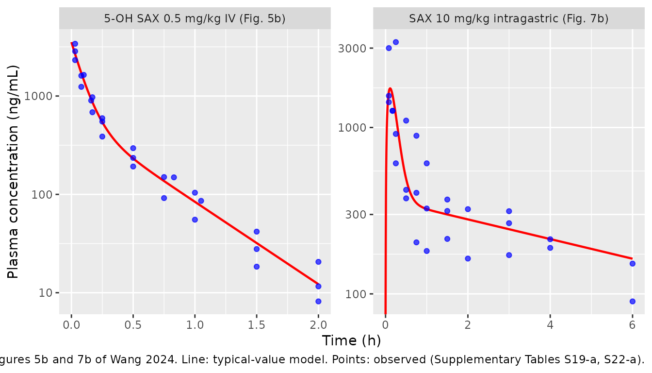
Replicating Figure 6b and Figure 8b (DPP-4 inhibition-time)
dplyr::bind_rows(
  sim_oh  |> dplyr::transmute(time, DPP4inh, panel = "5-OH SAX, total inhibition (Fig. 6b)"),
  sim_sax |> dplyr::filter(time <= 6) |>
    dplyr::transmute(time, DPP4inh, panel = "SAX, parent-attributed inhibition (Fig. 8b)")
) |>
  ggplot(aes(time, DPP4inh)) +
  geom_line(colour = "red", linewidth = 0.8) +
  geom_point(
    data = dplyr::bind_rows(
      obs_oh  |> dplyr::filter(!is.na(inh)) |>
        dplyr::transmute(time, DPP4inh = inh, panel = "5-OH SAX, total inhibition (Fig. 6b)"),
      obs_sax |> dplyr::filter(!is.na(inh_parent)) |>
        dplyr::transmute(time, DPP4inh = inh_parent, panel = "SAX, parent-attributed inhibition (Fig. 8b)")
    ),
    colour = "blue", alpha = 0.7
  ) +
  facet_wrap(~panel, scales = "free_x") +
  labs(x = "Time (h)", y = "DPP-4 inhibition ratio (%)",
       caption = "Replicates Figures 6b and 8b of Wang 2024. Line: typical-value model. Points: observed / derived (Supplementary Tables S19-a, S22-a).")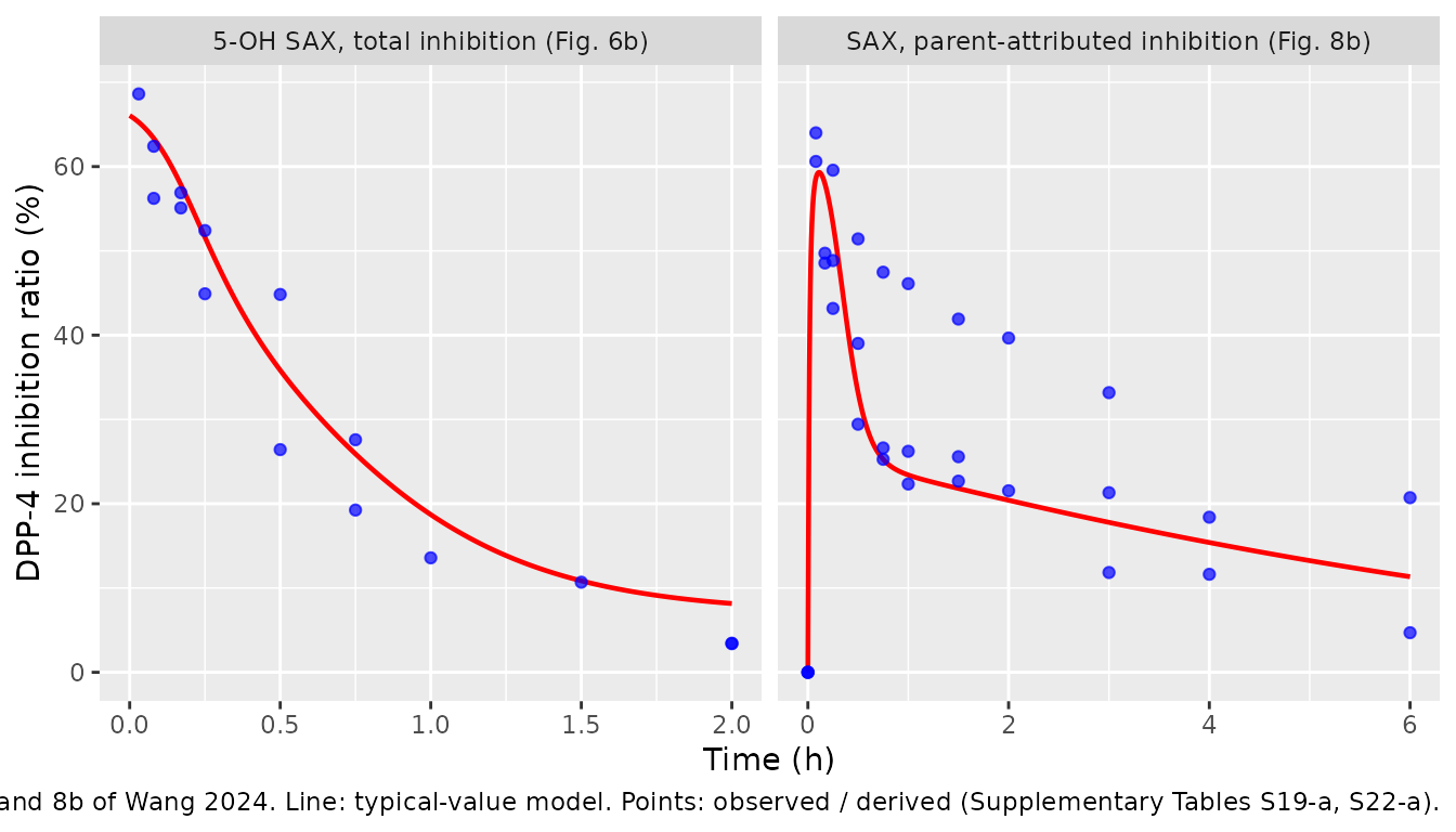
Replicating Figure 6c and Figure 8c (concentration-effect)
conc_grid <- 10^seq(0, 4, length.out = 200)
tibble::tibble(
  conc = rep(conc_grid, 2),
  drug = rep(c("5-OH SAX (Fig. 6c)", "SAX parent (Fig. 8c)"), each = length(conc_grid))
) |>
  dplyr::mutate(
    effect = dplyr::if_else(
      drug == "5-OH SAX (Fig. 6c)",
      7.03 + 60.88 * conc^1.31 / (251.74^1.31 + conc^1.31),
      71.47 * conc^1.38 / (544.74^1.38 + conc^1.38)
    )
  ) |>
  ggplot(aes(conc, effect, colour = drug)) +
  geom_line(linewidth = 0.8) +
  geom_vline(xintercept = c(251.74, 544.74), linetype = "dashed", alpha = 0.4) +
  scale_x_log10() +
  labs(x = "Plasma concentration (ng/mL)", y = "DPP-4 inhibition ratio (%)",
       colour = NULL,
       caption = "Replicates Figures 6c and 8c of Wang 2024. Dashed lines mark the two EC50 values.")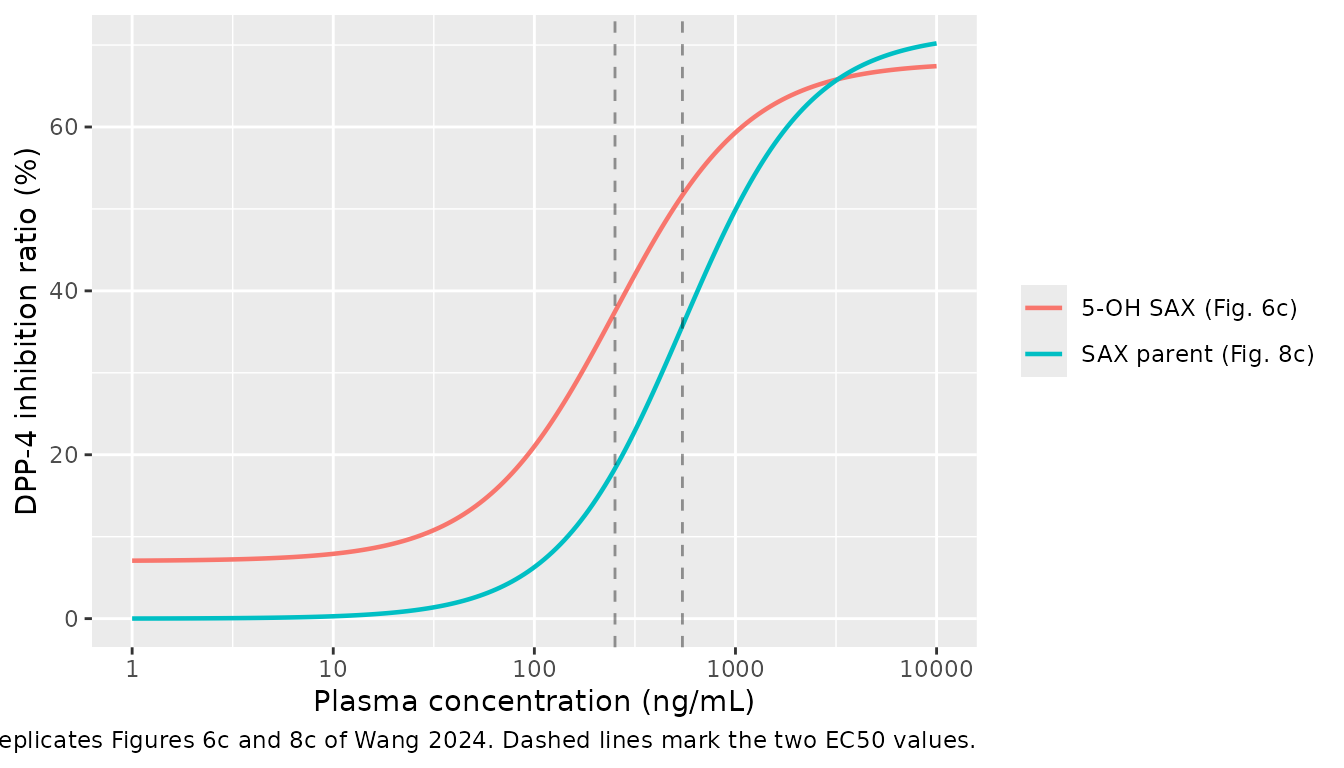
Replicating Figure 11 (total vs parent-attributed inhibition)
Figure 11 is the paper’s argument that the metabolite’s contribution cannot be ignored: after oral SAX, the measured total inhibition sits well above the share attributable to the parent alone.
obs_sax |>
  dplyr::select(rat, time, inh_total, inh_parent) |>
  tidyr::pivot_longer(c(inh_total, inh_parent), names_to = "series", values_to = "inh") |>
  dplyr::filter(!is.na(inh)) |>
  dplyr::mutate(series = dplyr::recode(
    series,
    inh_total  = "Total (SAX + 5-OH SAX), measured",
    inh_parent = "Parent SAX only, derived by subtraction"
  )) |>
  dplyr::group_by(series, time) |>
  dplyr::summarise(mean = mean(inh), sd = stats::sd(inh), .groups = "drop") |>
  ggplot(aes(time, mean, colour = series)) +
  geom_point() +
  geom_line() +
  geom_errorbar(aes(ymin = mean - sd, ymax = mean + sd), width = 0.1, na.rm = TRUE) +
  labs(x = "Time (h)", y = "DPP-4 inhibition ratio (%)", colour = NULL,
       caption = "Replicates Figure 11 of Wang 2024 (mean +/- SD, n = 3).")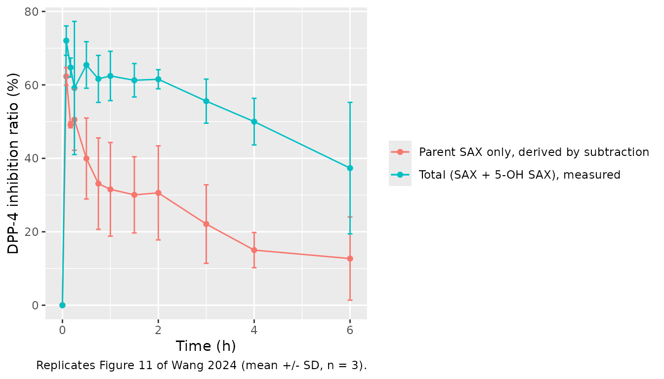
The paper’s central finding: EC50 ratio
ec50_oh  <- exp(oh_mod$theta[["lec50"]])
ec50_sax <- exp(sax_mod$theta[["lec50"]])
tibble::tibble(
  Quantity = c("EC50, 5-OH SAX (ng/mL)", "EC50, parent SAX (ng/mL)",
               "Ratio EC50(5-OH SAX) / EC50(SAX)", "Ratio reported by Wang 2024"),
  Value = c(round(ec50_oh, 2), round(ec50_sax, 2), round(ec50_oh / ec50_sax, 4), 0.46)
) |>
knitr::kable(caption = "The packaged models reproduce EC50(5-OH SAX) = 0.46 * EC50(SAX), i.e. the metabolite is about half as potent as the parent, confirming in vivo the in vitro literature value.")| Quantity | Value |
|---|---|
| EC50, 5-OH SAX (ng/mL) | 251.7400 |
| EC50, parent SAX (ng/mL) | 544.7400 |
| Ratio EC50(5-OH SAX) / EC50(SAX) | 0.4621 |
| Ratio reported by Wang 2024 | 0.4600 |
Assumptions and deviations
-
Kais derived, not tabulated. Table 11 reports only the absorption half-lifet1/2,Ka = 0.07 h. The model usesKa = log(2)/0.07 = 9.9021 1/h. Per-animal simulations uselog(2)/t1/2,Kafrom Supplementary Table S22-b. -
Fis assumed 1. Bioavailability appears in Eq 1 asF*Ka*Aabut is never estimated or reported, solfdepotisfixed(log(1))andCL,V,CL2andV2are apparent (CL/Fetc.). This is consistent with the paper’s own arithmetic: every animal’s tabulatedAUCequalsDose/CLexactly. -
No between-animal variability. Wang 2024 fitted
each rat individually in WinNonlin 8.1 and reported the mean and SD of
three individual estimates; no population model and no OMEGA were
estimated. The packaged models therefore carry no
etaterms. The reported SDs are preserved in the per-animal tables above rather than being converted into an invented OMEGA. Note in particular thatE0cannot be log-normal: the individual estimates run from -3.85% to 21.15%. -
PK residual error magnitude was never published.
Both PK models are described as additive, but no residual SD appears in
Table 9, Table 11, or the supplementary per-animal tables (the tabulated
stdev0belongs to the PD fit).addSdis thereforefixed(0)for both models and the PDaddSd_DPP4inhuses the publishedstdev0. -
The parent PD observations are derived, not
measured.
Wang_2024_saxagliptin_ratis fitted toIn_SAX = In_total - In_5OHSAX, where the second term comes from pushing the measured post-oral 5-OH SAX concentrations through the separately fitted metabolite model. SimulatedDPP4inhfrom this model is therefore the parent’s share of DPP-4 inhibition, not the observable total. -
e0is on the linear scale. Every other PD parameter is log-transformed, butE0takes a negative value in one of the three animals, so a log transform is not available. -
Typical-value predictions differ from the published means
for nonlinear summaries. The packaged
ini()holds the mean of each parameter, whereas Tables 9 and 11 report the mean of each derived quantity across animals. For quantities that are convex in the parameters these are not the same number. The clearest case is SAXCmax: the mean-parameter model gives about 1718 ng/mL against a published mean of 2197.13 ng/mL, because rat 2’s smallV(1081.89 mL/kg) produces a Cmax of 3587.55 ng/mL that pulls the arithmetic mean up. The same effect explains SAXt1/2beta(mean-parameter 5.09 h versus a published mean of 6.13 h, itself the mean of 3.82, 1.42 and 13.16 h). The per-animal comparison tables above are the strict check; they use each animal’s own parameters and match the published per-animal values closely. - Supplementary Tables S20 and S23 mix nominal and actual sampling times. Their row labels are a single nominal grid, but the per-animal predicted-concentration columns are evaluated at each animal’s actual bleed times, which differ between animals. A whole-table comparison is therefore not meaningful; the point-prediction check above uses the actual grid printed in Table S19-a and is restricted to one animal for that reason.
- Table S19-a rat 3 is column-shifted in the published PDF. That animal’s block prints its own actual sampling times against the concentration column and leaves the inhibition-ratio column unpopulated, so only rats 1 and 2 contribute observed 5-OH SAX inhibition ratios to the figures above.
- One published data point is internally inconsistent. In Table S22-a, rat 1 at 0.25 h has a total inhibition ratio (38.55%) below the parent-attributed ratio (48.85%), which the subtraction defining the parent series cannot produce. The value is reproduced as printed and not corrected.
- Only the early sampling window was modelled. Wang 2024 fitted the first 4 h (SAX) and first 2 h (5-OH SAX) of each profile. Simulations beyond those windows are extrapolations of the published model, not fitted predictions.