Tacrolimus intracellular calcineurin inhibition (Fontova 2023)
Source:vignettes/articles/Fontova_2023_tacrolimus.Rmd
Fontova_2023_tacrolimus.RmdModel and source
Fontova 2023 measured tacrolimus inside peripheral blood mononuclear cells (PBMCs) and calcineurin (CN) activity in the same cells over a 24 h steady-state dosing interval, first on twice-daily immediate-release tacrolimus (TAC-IR) and again four weeks after conversion to once-daily extended-release tacrolimus (TAC-LCP). The pharmacokinetics was analysed non-compartmentally. The one fitted model is a naive-pooled direct inhibitory Imax model without baseline (Hill coefficient 1) linking the intracellular concentration to CN activity, pooled over both formulations:
where is the intracellular tacrolimus concentration (pg/million cells) and is the percentage by which a patient’s CN activity exceeds that patient’s own nadir CN activity (the paper’s “% inhibition Inadir”, Equation 2, ). is largest with no drug and falls towards the nadir as the concentration rises.
Fontova_2023_tacrolimus encodes this model. It has no PK
component: the intracellular concentration is supplied per observation
row as the covariate CONC_TACROLIMUS_PGMC.
- Citation: Fontova P, Colom H, Rigo-Bonnin R, Bestard O, Vidal-Alabro A, van Merendonk LN, Cerezo G, Polo C, Montero N, Melilli E, Coloma A, Manonelles A, Cruzado JM, Grinyo JM, Lloberas N. The Effect of Intracellular Tacrolimus Exposure on Calcineurin Inhibition in Immediate- and Extended-Release Tacrolimus Formulations. Pharmaceutics 2023;15(5):1481. doi:10.3390/pharmaceutics15051481.
- Article: https://doi.org/10.3390/pharmaceutics15051481
Population
Twenty-five stable adult kidney transplant recipients were enrolled at Bellvitge University Hospital, Spain (NCT02961608, 2016-2018). They had been transplanted at least six months earlier (median 1.84 years) and had whole-blood tacrolimus C0 of 5-10 ng/mL at steady state; 23 completed both intracellular profiles (Results 3.1). In the enrolled cohort (Table 1), 72% were male, median age was 58.8 years (IQR 48.4-71.1) and median weight 73.0 kg (IQR 62.8-79.9). Twenty (80%) were CYP3A5 *3/*3 non-expressers. The median total daily dose was 3.0 mg on TAC-IR and 2.0 mg on TAC-LCP after a 1:0.7 conversion. Doses were taken fasting.
The same information is available programmatically as
readModelDb("Fontova_2023_tacrolimus")$population.
Source trace
| Element | Value | Source location |
|---|---|---|
| Model form, inhibitory Imax without baseline | E = e0 * (1 - C / (ic50 + C)) |
Methods 2.4.2 Equation 4; Results 3.4 |
| Hill coefficient | 1 (simple Imax selected over sigmoid) | Results 3.4; Discussion |
| Response definition | 100 * (I - I_nadir) / I_nadir |
Methods 2.4.1 Equation 2 |
le0 |
log(30.4) percent | Results 3.4; Discussion |
lic50 |
log(43.9) pg/million cells | Abstract; Results 3.4; Discussion |
addSd |
0, not reported | Methods 2.4.2 names FOCE-I only |
| IIV | none (naive-pooled fit) | Methods 2.4.2 |
Covariate CONC_TACROLIMUS_PGMC
|
intracellular PBMC tacrolimus | Methods 2.2; Equation 4 C
|
| Intracellular and CN geometric-mean profiles used below | digitised | Figure 2C |
| Published NCA of intracellular tacrolimus | C0, Cmax, AUC0-24 | Table 2 |
Concentration-response
mod <- readModelDb("Fontova_2023_tacrolimus")
ui <- rxode2::rxode2(mod)
e0 <- exp(ui$theta[["le0"]])
ic50 <- exp(ui$theta[["lic50"]])

# The model is algebraic (no ODE state), so a single "subject" walks the
# concentration grid; time only orders the rows.
conc_grid <- c(0, seq(1, 450, by = 1))
ev_grid <- data.frame(
  id = 1L,
  time = seq_along(conc_grid),
  evid = 0L,
  amt = 0,
  CONC_TACROLIMUS_PGMC = conc_grid
)
sim_grid <- rxode2::rxSolve(mod, events = ev_grid, keep = "CONC_TACROLIMUS_PGMC") |>
  as.data.frame()
The closed form fixes two anchors exactly: the response is with no drug and at . The two sides of this check use the same parameters, so the bound is tight.
at_conc <- function(sim, conc) {
  sim$calcineurin_pct_above_nadir[match(conc, sim$CONC_TACROLIMUS_PGMC)]
}
stopifnot(
  abs(at_conc(sim_grid, 0) - 30.4) < 1e-8,
  abs(at_conc(sim_grid, 44) - 30.4 * 43.9 / (43.9 + 44)) < 1e-8,
  abs(e0 / 2 - 30.4 * (1 - 43.9 / (2 * 43.9))) < 1e-8
)
Figure 2D and Figure 2E
Figure 2E plots the observed against the predicted response. Its predicted values lie between about 3 and 26 percent over the observed intracellular concentrations of about 5 to 420 pg/million cells (Figure 2D x-axis). The model reproduces that range.
pred_range <- range(at_conc(sim_grid, c(5, 420)))
pred_range
#> [1]  2.876827 27.291616
stopifnot(
  abs(pred_range[1] - 3) < 1,
  abs(pred_range[2] - 26) < 2
)
The solid “mean predicted” line printed in Figure 2D does not match the reported . Tracing the line off the figure gives the points below. A straight-line fit of against recovers , within 1% of the reported 43.9, but with rather than 30.4. The text value is stated twice (Results 3.4 and Discussion) and agrees with Figure 2E’s predicted range. The model therefore uses 30.4, and the Figure 2D line is treated as a plotting error (see Assumptions and deviations).
# Maintainers' trace of the Figure 2D solid line (percent above nadir).
fig2d_line <- data.frame(
  conc = c(10, 25, 50, 75, 100, 150, 200, 300, 400),
  pct = c(65.9, 51.9, 37.8, 30.0, 24.8, 18.1, 14.4, 10.2, 8.0)
)
fit_line <- lm(I(1 / pct) ~ conc, data = fig2d_line)
line_e0 <- 1 / coef(fit_line)[[1]]
line_ic50 <- coef(fit_line)[[1]] / coef(fit_line)[[2]]
c(line_e0 = line_e0, line_ic50 = line_ic50)
#>   line_e0 line_ic50
#>  81.12981  43.48153
stopifnot(abs(line_ic50 - 43.9) / 43.9 < 0.1)

ggplot(sim_grid, aes(CONC_TACROLIMUS_PGMC, calcineurin_pct_above_nadir)) +
  geom_line(aes(colour = "Model (E0 = 30.4, IC50 = 43.9)"), linewidth = 1) +
  geom_point(
    data = fig2d_line,
    aes(conc, pct, colour = "Figure 2D printed line (traced)")
  ) +
  labs(
    x = "Intracellular tacrolimus (pg/million cells)",
    y = "CN activity above nadir (%)",
    colour = NULL,
    caption = "Replicates the model curve of Figure 2D of Fontova 2023."
  ) +
  theme_bw() +
  theme(legend.position = "bottom")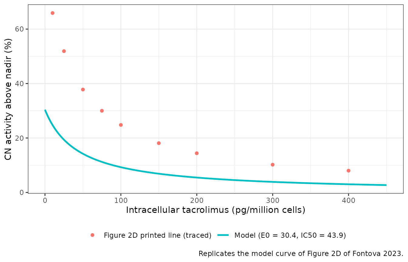
Time course over the dosing interval
Figure 2C shows the geometric-mean intracellular tacrolimus and CN activity over 24 h on each formulation. The maintainers digitised both from the figure. The intracellular profile includes a 13.5 h point that is plotted but missing from the Methods sampling list. Driving the model with the mean concentration profile gives the typical response at each time.
# Digitised from Fontova 2023 Figure 2C. Intracellular tacrolimus in
# pg/million cells (left axis); CN activity in pmol RII/min/mg protein
# (right axis).
fig2c <- tibble::tribble(
  ~time, ~conc_IR, ~conc_LCP, ~cna_IR, ~cna_LCP,
  0,     26,       26,        280,     270,
  0.5,   38,       28,        260,     256,
  1,     62,       30.5,      247.5,   249,
  1.5,   76,       32,        237.5,   246,
  2,     76,       36,        239,     233,
  3,     63,       48,        237.5,   237.5,
  4,     57,       60,        250,     230.6,
  6,     48,       59.5,      267.5,   229,
  8,     41,       52.5,      284,     234,
  12,    31.5,     41.5,      292.5,   247.5,
  12.5,  35,       40,        267.5,   247.5,
  13,    41,       39,        261,     257.5,
  13.5,  48,       38,        251,     253,
  14,    47,       35.5,      254,     256,
  15,    50,       35,        256,     262,
  20,    32,       30,        266,     266,
  24,    27,       25.5,      283,     283
) |>
  tidyr::pivot_longer(
    -time,
    names_to = c(".value", "treatment"),
    names_sep = "_"
  ) |>
  mutate(
    treatment = recode(treatment, IR = "TAC-IR", LCP = "TAC-LCP"),
    id = as.integer(factor(treatment))
  )

# One solve per formulation: the model has no random effects, and rxode2
# warns on a multi-subject solve without an omega matrix.
sim_tc <- lapply(split(fig2c, fig2c$treatment), function(d) {
  ev <- transmute(d, id = 1L, time, evid = 0L, amt = 0, CONC_TACROLIMUS_PGMC = conc)
  rxode2::rxSolve(mod, events = ev, keep = "CONC_TACROLIMUS_PGMC") |>
    as.data.frame() |>
    mutate(treatment = d$treatment[1])
}) |>
  bind_rows() |>
  left_join(select(fig2c, treatment, time, cna), by = c("treatment", "time"))
The model predicts the lowest CN activity at the intracellular peak, with no delay. Figure 2C shows the same, and the paper reports no delay between peak concentration and maximum inhibition (Results 3.3). Across the 17 sampling times, the predicted response and the observed geometric-mean CN activity should therefore rise and fall together.
tc_cor <- sim_tc |>
  group_by(treatment) |>
  summarise(
    spearman = cor(calcineurin_pct_above_nadir, cna, method = "spearman"),
    .groups = "drop"
  )
knitr::kable(tc_cor, digits = 2, caption = "Rank correlation between the predicted response and the digitised geometric-mean CN activity.")| treatment | spearman |
|---|---|
| TAC-IR | 0.87 |
| TAC-LCP | 0.80 |
sim_tc |>
  select(treatment, time, `Model: CN activity above nadir (%)` = calcineurin_pct_above_nadir,
         `Figure 2C: CN activity (pmol RII/min/mg prot)` = cna,
         `Figure 2C: intracellular tacrolimus (pg/million cells)` = CONC_TACROLIMUS_PGMC) |>
  tidyr::pivot_longer(-c(treatment, time)) |>
  ggplot(aes(time, value, colour = treatment)) +
  geom_line() +
  geom_point() +
  facet_wrap(~name, ncol = 1, scales = "free_y") +
  scale_x_continuous(breaks = seq(0, 24, 4)) +
  labs(
    x = "Time after morning dose (h)", y = NULL, colour = NULL,
    caption = "Replicates the PD time course of Figure 2C of Fontova 2023 with the model response."
  ) +
  theme_bw() +
  theme(legend.position = "bottom")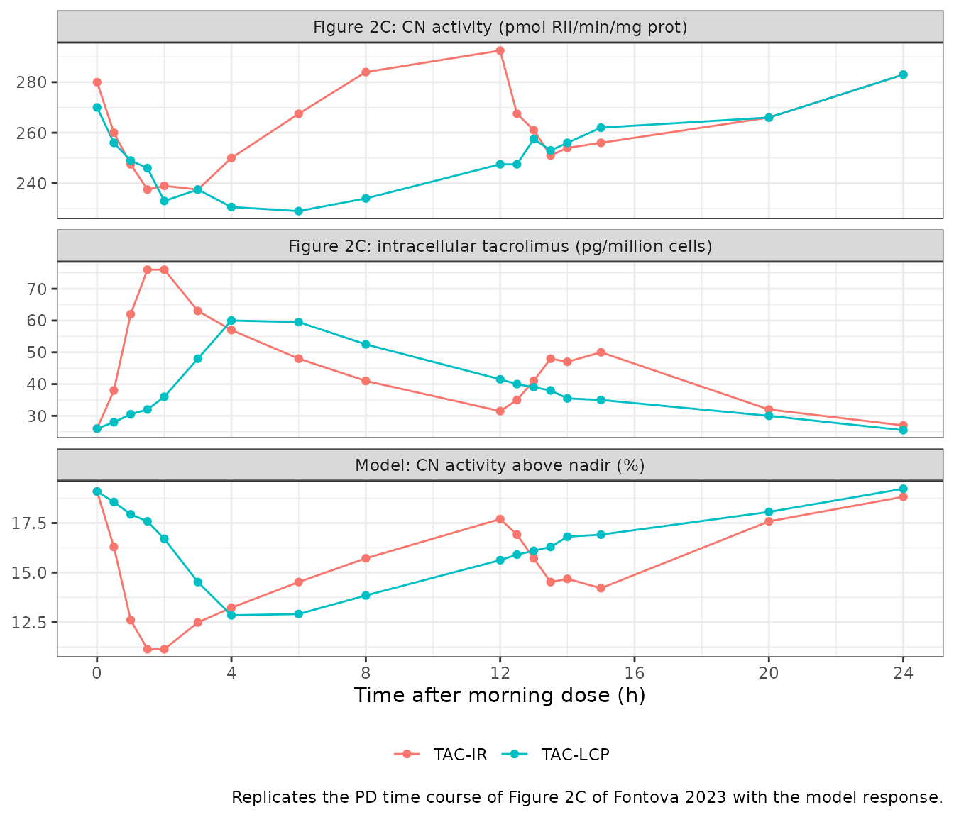
The model response is a per-patient nadir-normalised percentage, while Figure 2C plots absolute CN activity averaged over patients. The two are compared on timing and direction, not on level. The swing of the mean CN profile above its own minimum (about 23% on both formulations) is the same order as . The Discussion attributes this modest E0 to a rate-limited CN inhibition.
NCA of the driving profiles
The model has no PK component, so NCA here checks the digitised intracellular input against the published NCA (Table 2). An NCA of the geometric-mean curve is not the same as the geometric mean of per-patient NCA. Individual peaks occur at different times and are blunted by averaging, so the curve’s Cmax is expected to fall below the published geometric-mean Cmax. AUC and the troughs should agree closely.
conc_nca <- fig2c |>
  select(id, treatment, time, conc)
stopifnot(any(conc_nca$time == 0))

intervals <- data.frame(start = 0, end = 24, cmax = TRUE, tmax = TRUE, auclast = TRUE)
nca_res <- PKNCA::pk.nca(
  PKNCA::PKNCAdata(
    PKNCA::PKNCAconc(conc_nca, conc ~ time | treatment + id),
    intervals = intervals
  )
)
#> No dose information provided, calculations requiring dose will return NA.

published <- tibble::tribble(
  ~treatment, ~cmax,  ~auclast, ~tmax,
  "TAC-IR",   93.06,  1052.69,  1.53,
  "TAC-LCP",  70.65,  969.45,   6.00
)

cmp <- nlmixr2lib::ncaComparisonTable(
  simulated = nca_res,
  reference = published,
  by = "treatment",
  units = c(cmax = "pg/million cells", auclast = "pg/million cells*h", tmax = "h"),
  tolerance_pct = 20
)
cmp |>
  dplyr::rename("Formulation" = treatment) |>
  knitr::kable(
    caption = paste(
      "NCA of the digitised Figure 2C geometric-mean intracellular profile",
      "versus Fontova 2023 Table 2 (Cmax, AUC0-24: geometric means; Tmax: median).",
      "* differs by more than 20%."
    ),
    digits = 2
)| NCA parameter | Formulation | Reference | Simulated | % diff |
|---|---|---|---|---|
| Cmax (pg/million cells) | TAC-IR | 93.1 | 76 | -18.3% |
| Cmax (pg/million cells) | TAC-LCP | 70.6 | 60 | -15.1% |
| Tmax (h) | TAC-IR | 1.53 | 1.5 | -2.0% |
| Tmax (h) | TAC-LCP | 6 | 4 | -33.3%* |
| AUClast (pg/million cells*h) | TAC-IR | 1050 | 1030 | -2.2% |
| AUClast (pg/million cells*h) | TAC-LCP | 969 | 961 | -0.9% |
auc_sim <- as.data.frame(nca_res) |>
  filter(PPTESTCD == "auclast") |>
  left_join(published, by = "treatment")
stopifnot(all(abs(auc_sim$PPORRES / auc_sim$auclast - 1) < 0.15))
AUC0-24 of the mean curve agrees with the published geometric means to within a few percent on both formulations. The digitised troughs (26 and 26 pg/million cells at 0 h; 27 and 25.5 at 24 h) match Table 2’s C0 (26.78, 25.63) and C24 (27.09, 25.28). Cmax of the mean curve is below the published geometric-mean Cmax, as expected from averaging over patients with different Tmax. The TAC-LCP Tmax of the mean curve (4 h) is earlier than the published median of 6 h, because the mean curve is flat between 4 and 6 h.
Assumptions and deviations
-
E0 conflict between text and Figure 2D. The text
gives E0 = 30.4% (Results 3.4 and Discussion), and Figure 2E’s predicted
values (about 3 to
- agree with it. The solid line printed in Figure 2D, traced above, has the same IC50 of 43.9 but an E0 near 81. The maintainers ruled that the text value applies and treat the Figure 2D line as a plotting error.
-
Residual error not reported. The paper names the
estimation method (FOCE-I) but not the residual-error model or its
magnitude.
addSdis held at 0, so simulations return the typical response. - No inter-individual variability. The fit was naive-pooled, so the model has no random effects. The paper notes high variability in the data (Discussion; Figure 2D scatter) but gives no estimate of it.
-
PD-only. Fontova 2023 did not fit a PK model;
whole-blood and intracellular pharmacokinetics were analysed
non-compartmentally. To drive this model from a dosing regimen, supply
intracellular PBMC concentrations in pg/million cells from another
source. Per-volume PBMC concentrations, such as the
Cpbmcoutput ofAgergaard_2025_tacrolimus, are on a different basis and cannot be converted without a per-cell volume. - Pooled formulations. One model describes both TAC-IR and TAC-LCP. The formulation difference in CN response comes entirely from the different intracellular concentration-time profiles, so formulation is not a model covariate.
- Digitised inputs. The time-course and NCA sections use geometric-mean profiles digitised by the maintainers from Figure 2C. They serve as illustrations and input checks, not as published parameter values.
-
Response wording. The paper calls the response “%
inhibition Inadir”, but larger values mean less
inhibition (activity further above the patient’s nadir). The output is
named
calcineurin_pct_above_nadirto avoid that inversion.