Dabigatran coagulation-time PD (Fuhr 2020)
Source:vignettes/articles/Fuhr_2020_dabigatran.Rmd
Fuhr_2020_dabigatran.RmdModel and source
- Citation: Fuhr LM, Hanke N, Meibohm B, Lehr T. (2020). Effective Removal of Dabigatran by Idarucizumab or Hemodialysis: A Physiologically Based Pharmacokinetic Modeling Analysis. Clinical Pharmacokinetics 59:809-825. doi:10.1007/s40262-019-00857-y. PD equations from Electronic Supplementary Material 1, section ‘Pharmacodynamic modeling’, Equations 16-19.
- Description: Direct concentration-effect pharmacodynamic model relating the unbound sum dabigatran plasma concentration (unbound dabigatran plus unbound dabigatran acyl-glucuronide, i.e. drug bound neither to plasma proteins nor to idarucizumab) to four coagulation times in adults: activated partial thromboplastin time (aPTT) and thrombin time (TT) as a combined linear plus Emax function, and diluted thrombin time (dTT) and ecarin clotting time (ECT) as linear functions (Fuhr 2020 ESM Equations 16-19). Only this PD layer is reproduced here. The idarucizumab and dabigatran whole-body PBPK layers, the idarucizumab-dabigatran binding model and the hemodialysis extension were built in the PK-Sim / MoBi platform and depend on platform-database organ volumes, blood flows and partition coefficients that the paper does not print, so they are not reproduced (see the vignette ‘Assumptions and deviations’). The unbound sum dabigatran concentration is therefore supplied by the user as the time-varying covariate CU_DABIGATRAN_UM. No inter-individual variability and no residual-error model are reported (the PD data were digitised study-arm means), so both are encoded as zero.
- Article: https://doi.org/10.1007/s40262-019-00857-y (open access, PMC7292816)
Fuhr 2020 describes how dabigatran is reversed by its antidote idarucizumab and by hemodialysis. The analysis has five parts:
- a whole-body PBPK model of idarucizumab, including an extended kidney with megalin-mediated tubular reabsorption;
- the idarucizumab-dabigatran binding interaction (Kd 2.1 pmol/L), merged with the authors’ earlier dabigatran PBPK model;
- a hemodialysis extension with a dialyzer compartment;
- a direct concentration-effect PD model linking the unbound sum dabigatran plasma concentration to four coagulation times (aPTT, dTT, ECT and TT);
- simulations of reversal scenarios.
Parts 1-3 were built in PK-Sim / MoBi (Open Systems Pharmacology
Suite 8.0). Only part 4, the PD layer, is packaged in
nlmixr2lib. The reasons are in Assumptions and deviations. The
PD layer does not depend on the PBPK model’s structure. Its only input
is the unbound sum dabigatran concentration, which you supply as the
time-varying covariate CU_DABIGATRAN_UM (umol/L). You can
take it from any dabigatran PK model or from measured
concentrations.
Population
The PD equations were fitted to digitised study-arm means pooled from 26 dabigatran-treated arms of three clinical programmes (Fuhr 2020 ESM Table S8):
- Glund 2015: healthy Caucasian men.
- Glund 2016 / 2017: middle-aged (45-64 years) and elderly (65-80 years) Caucasians, and Caucasians with mild or moderate renal impairment.
- Yasaka 2017: healthy Japanese men.
All subjects received steady-state oral dabigatran etexilate: 220 mg twice daily, or 150 mg twice daily in renal impairment, for 3.5 days. Most arms then received intravenous idarucizumab (1000-7500 mg), and the fitted data include coagulation measurements both before and after the antidote. Across the Table 1 arms, mean age was 24-72 years, mean weight 57-90 kg and mean creatinine clearance 59-139 mL/min. The number of individuals behind the PD fit is not reported.
Source trace
| Model element | Value | Source |
|---|---|---|
Driver CU_DABIGATRAN_UM = unbound dabigatran + unbound
glucuronide |
umol/L | ESM Eq. 3; main text 2.3 |
| aPTT = Emax * C / (EC50 + C) + slope * C + baseline | ESM Eq. 16; main text 3.4 | |
lrbase_aPTT |
30.21 s | ESM Eq. 16 |
lemax_aPTT |
17.94 s | ESM Eq. 16 |
lec50_aPTT |
0.04 umol/L | ESM Eq. 16 |
lslope_aPTT |
61.67 s per umol/L | ESM Eq. 16 |
| dTT = slope * C + baseline | ESM Eq. 17 | |
lrbase_dTT |
31.59 s | ESM Eq. 17 |
lslope_dTT |
88.30 s per umol/L | ESM Eq. 17 |
| ECT = slope * C + baseline | ESM Eq. 18 | |
lrbase_ECT |
34.85 s | ESM Eq. 18 |
lslope_ECT |
209.70 s per umol/L | ESM Eq. 18 |
| TT = Emax * C / (EC50 + C) + slope * C + baseline | ESM Eq. 19; main text 3.4 | |
lrbase_TT |
12.93 s | ESM Eq. 19 |
lemax_TT |
106.28 s | ESM Eq. 19 |
lec50_TT |
0.19 umol/L | ESM Eq. 19 |
lslope_TT |
144.02 s per umol/L | ESM Eq. 19 |
addSd_aPTT, addSd_dTT,
addSd_ECT, addSd_TT
|
0 (fixed) | not reported |
Concentration-effect curves
mod <- rxode2::rxode2(readModelDb("Fuhr_2020_dabigatran"))

mw_dab <- 471.5 # g/mol; the ESM rounds it to 472

conc_ngml <- seq(0, 220, by = 2)
conc_grid <- data.frame(
  id = 1L,
  time = seq_along(conc_ngml) - 1,
  evid = 0L,
  amt = 0,
  dvid = 1L,
  conc_ngml = conc_ngml
) |>
  mutate(CU_DABIGATRAN_UM = conc_ngml / mw_dab)

sim <- rxode2::rxSolve(
  mod,
  events = conc_grid,
  omega = NA,
  sigma = NA,
  keep = "conc_ngml",
  returnType = "data.frame"
)

sim_long <- sim |>
  dplyr::select(conc_ngml, aPTT, dTT, ECT, TT) |>
  tidyr::pivot_longer(-conc_ngml, names_to = "assay", values_to = "seconds") |>
  mutate(assay = factor(assay, levels = c("aPTT", "dTT", "ECT", "TT")))
# Replicates Figure 6 (left column) of Fuhr 2020: coagulation times versus the
# unbound sum dabigatran plasma concentration.
ggplot(sim_long, aes(conc_ngml, seconds, colour = assay)) +
  geom_line(linewidth = 1) +
  facet_wrap(~assay, scales = "free_y") +
  labs(
    x = "Unbound sum dabigatran plasma concentration (ng/mL)",
    y = "Coagulation time (s)",
    caption = "Replicates Figure 6 (left column) of Fuhr 2020."
  ) +
  theme_bw() +
  theme(legend.position = "none")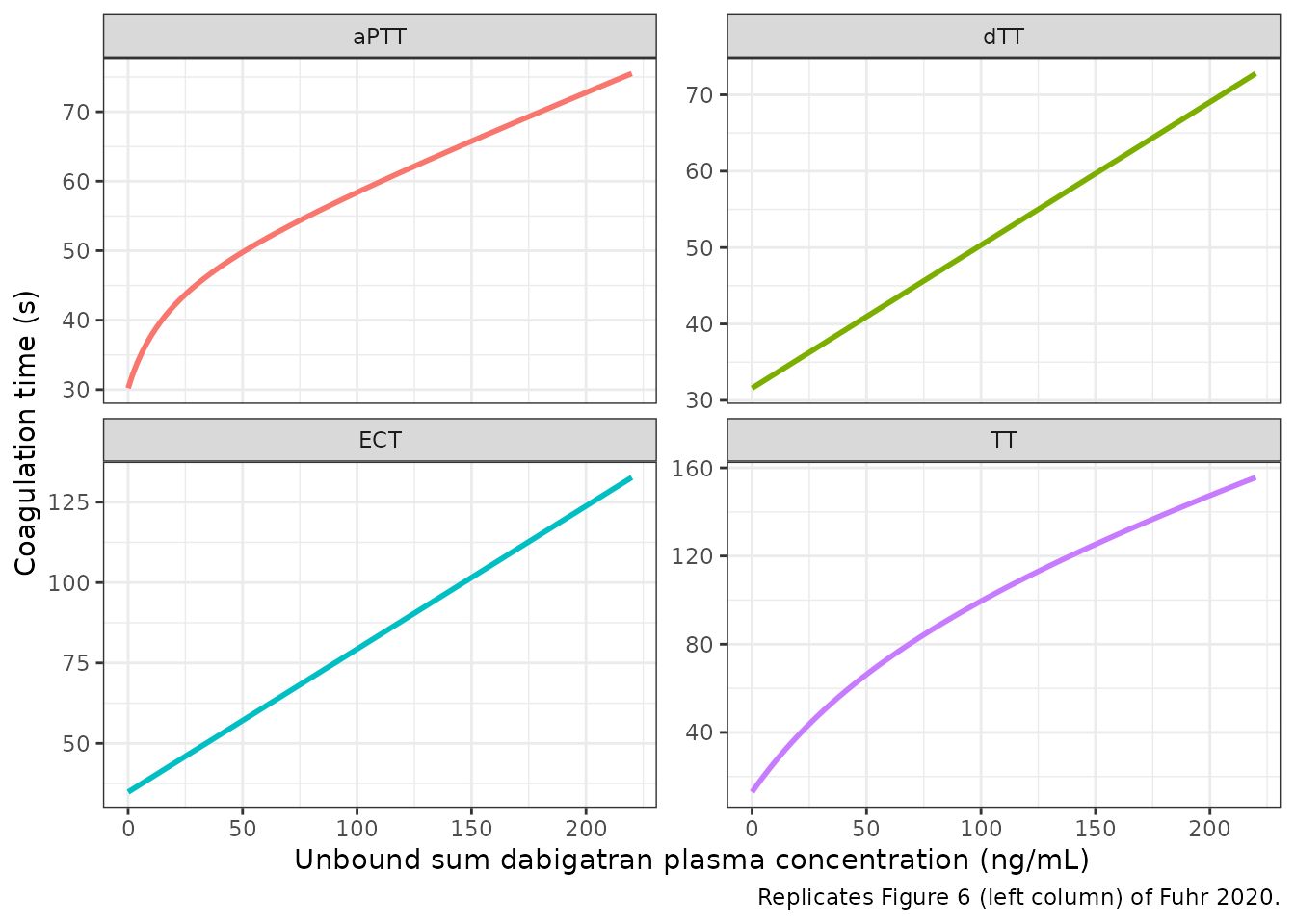
Validation
The PD layer is a set of closed-form equations with no dosing, so NCA does not apply. The model is checked in three ways instead.
Baselines at zero concentration
With no dabigatran, every assay must return its intercept exactly. This checks the transcription of the four baselines.
at0 <- sim |> dplyr::filter(conc_ngml == 0)
stopifnot(
  isTRUE(all.equal(at0$aPTT, 30.21)),
  isTRUE(all.equal(at0$dTT, 31.59)),
  isTRUE(all.equal(at0$ECT, 34.85)),
  isTRUE(all.equal(at0$TT, 12.93))
)
at0 |> dplyr::select(aPTT, dTT, ECT, TT) |> knitr::kable(digits = 2)| aPTT | dTT | ECT | TT |
|---|---|---|---|
| 30.21 | 31.59 | 34.85 | 12.93 |
Agreement with the published fitted curves (unit check)
The ESM gives the concentration unit only in its definition of the driver (Equation 3, umol/L), while Figure 6 plots the curves against ng/mL. The maintainers read the published fitted lines off Figure 6 at 100 and 220 ng/mL, to about +/- 2 s. If the equations had been in ng/mL or nmol/L, the predictions would be off by orders of magnitude, so agreement here confirms the umol/L reading and the dabigatran molecular-weight conversion.
fig6 <- data.frame(
  conc_ngml = rep(c(100, 220), each = 4),
  assay = rep(c("aPTT", "dTT", "ECT", "TT"), 2),
  figure6_s = c(59, 50, 80, 98, 75, 72, 132, 155)
)

chk <- fig6 |>
  left_join(sim_long |> mutate(assay = as.character(assay)), by = c("conc_ngml", "assay")) |>
  mutate(pct_diff = 100 * (seconds - figure6_s) / figure6_s)

chk |>
  dplyr::rename(
    "Unbound sum DAB (ng/mL)" = conc_ngml,
    "Assay" = assay,
    "Figure 6 curve (s)" = figure6_s,
    "Model (s)" = seconds,
    "Difference (%)" = pct_diff
  ) |>
knitr::kable(digits = 1)| Unbound sum DAB (ng/mL) | Assay | Figure 6 curve (s) | Model (s) | Difference (%) |
|---|---|---|---|---|
| 100 | aPTT | 59 | 58.4 | -1.0 |
| 100 | dTT | 50 | 50.3 | 0.6 |
| 100 | ECT | 80 | 79.3 | -0.8 |
| 100 | TT | 98 | 99.5 | 1.6 |
| 220 | aPTT | 75 | 75.5 | 0.7 |
| 220 | dTT | 72 | 72.8 | 1.1 |
| 220 | ECT | 132 | 132.7 | 0.5 |
| 220 | TT | 155 | 155.7 | 0.4 |
Cross-assay consistency in the individual profile
The middle column of Figure 6 shows the four model-predicted coagulation times for healthy Japanese subjects on 220 mg dabigatran etexilate twice daily, before and after 1000 mg idarucizumab at 242 h. All four curves come from one predicted concentration, so the peak just before idarucizumab must map to a single concentration under all four equations. The maintainers read the ECT peak as about 115 s. Inverting Equation 18 gives the concentration, from which the other three assays follow. The Figure 6 peaks for comparison are about 70 s (aPTT), 65 s (dTT) and 145 s (TT).
c_peak <- (115 - 34.85) / 209.70 # umol/L, from the ECT peak
peak <- rxode2::rxSolve(
  mod,
  events = data.frame(id = 1L, time = 0, evid = 0L, amt = 0, dvid = 1L, CU_DABIGATRAN_UM = c_peak),
  omega = NA,
  sigma = NA,
  returnType = "data.frame"
)
peak_chk <- data.frame(
  assay = c("aPTT", "dTT", "TT"),
  figure6_s = c(70, 65, 145),
  model_s = c(peak$aPTT, peak$dTT, peak$TT)
) |>
  mutate(pct_diff = 100 * (model_s - figure6_s) / figure6_s)
knitr::kable(peak_chk, digits = 1)| assay | figure6_s | model_s | pct_diff |
|---|---|---|---|
| aPTT | 70 | 70.0 | 0.0 |
| dTT | 65 | 65.3 | 0.5 |
| TT | 145 | 139.0 | -4.2 |
After idarucizumab, Figure 6 shows every assay falling to its baseline (about 31, 31, 35 and 13 s). This matches the zero-concentration values above, which is expected because idarucizumab captures essentially all unbound dabigatran.
Illustrative time course
The model needs a concentration trajectory. As a demonstration only, this section takes the typical-value total dabigatran profile from the Yang 2024 popPK model in nlmixr2lib (healthy Chinese adults, fasted, ABCB1 rs4148738 non-CT). It runs 220 mg twice daily for 3.5 days (seven doses, as in the Fuhr 2020 studies) and converts the result to unbound concentrations with fu = 0.65 (35% protein binding, Fuhr 2020 Introduction). This is not the Fuhr 2020 PBPK prediction. Yang 2024 was fitted to single 150 mg doses, and its total dabigatran may not match the hydrolysed “sum” moiety.
pk <- rxode2::rxode2(readModelDb("Yang_2024_dabigatran"))
#> ℹ parameter labels from comments will be replaced by 'label()'
pk_ev <- rxode2::et(amt = 220, cmt = "depot", ii = 12, addl = 6) |>
  rxode2::et(seq(0, 96, by = 0.25), cmt = "central") |>
  as.data.frame() |>
  mutate(FED_HIGHFAT = 0, SNP_ABCB1_RS4148738_HET = 0)
pk_sim <- rxode2::rxSolve(pk, events = pk_ev, omega = NA, sigma = NA, returnType = "data.frame")

pd_ev <- data.frame(
  id = 1L,
  time = pk_sim$time,
  evid = 0L,
  amt = 0,
  dvid = 1L,
  CU_DABIGATRAN_UM = 0.65 * pk_sim$Cc / mw_dab
)
pd_sim <- rxode2::rxSolve(mod, events = pd_ev, omega = NA, sigma = NA, returnType = "data.frame")

pd_sim |>
  dplyr::select(time, aPTT, dTT, ECT, TT) |>
  tidyr::pivot_longer(-time, names_to = "assay", values_to = "seconds") |>
  ggplot(aes(time, seconds, colour = assay)) +
  geom_line(linewidth = 0.8) +
  facet_wrap(~assay, scales = "free_y") +
  labs(
    x = "Time (h)",
    y = "Coagulation time (s)",
    caption = "Illustrative only: Yang 2024 typical PK, fu = 0.65, driving Fuhr 2020 PD."
  ) +
  theme_bw() +
  theme(legend.position = "none")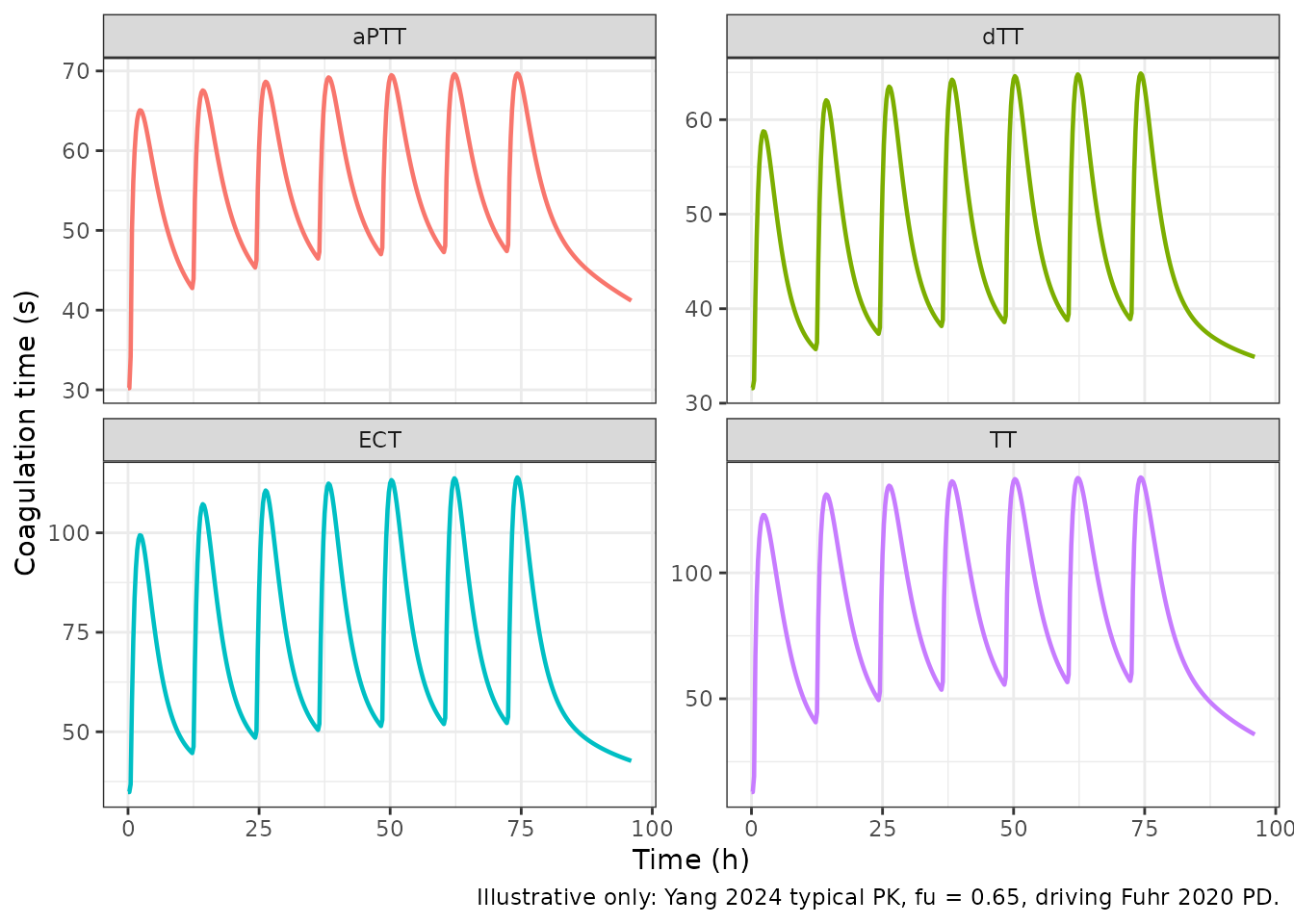
Assumptions and deviations
The PBPK, binding and dialysis layers are not packaged
The idarucizumab and dabigatran PBPK models run on the PK-Sim / MoBi platform. Their organ volumes, blood flows, surface areas and tissue partition coefficients come from the platform’s physiology database for each simulated individual and are not printed in the paper or the ESM. The ESM prints the drug-specific parameters (Table 2 and Table S3), the kidney-extension equations (ESM Eq. 5-13), the binding kinetics (ESM Eq. 14-15) and the dialyzer clearance (main text Eq. 2, with KoA from Liesenfeld 2013). The whole-body structure they plug into cannot be rebuilt from the publication, so these layers are not reproduced. The binding and dialysis parts act on platform-computed plasma and interstitial concentrations, so they cannot be separated from the PBPK model either.
A dabigatran hemodialysis model with the same dialysis-clearance form
is available as Liesenfeld_2013_dabigatran.
Driver definition
CU_DABIGATRAN_UM is the unbound sum of dabigatran and
its acyl-glucuronide. It excludes drug bound to plasma proteins and drug
bound to idarucizumab. This matches the assays in the source studies,
which hydrolysed the glucuronide and ultrafiltered the sample. A total
plasma concentration must be multiplied by the unbound fraction (about
0.65) before use. A value in ng/mL must be divided by 471.5.
No IIV and no residual error
The paper fitted the equations to digitised study-arm means and reports only point estimates, with no standard errors, inter-individual variability or residual-error model. Performance is summarised as mean relative deviation (1.16, 1.11, 1.16 and 1.27 for aPTT, dTT, ECT and TT). All four additive residual SDs are therefore fixed at zero. Free them when refitting to individual data.