Islatravir in rats (Kinsale 2024)
Source:vignettes/articles/Kinsale_2024_islatravir_rat.Rmd
Kinsale_2024_islatravir_rat.RmdModel and source
- Citation: Kinsale TS, Cottrell ML, Li L, Brand R, Gatto G, Luecke E, Norton C, Krovi A, Dumond JB, Rao G, Yeshwante S, Van Horne B, Van Der Straten A, Kashuba ADM, Johnson LM. Pharmacokinetic Modeling to Guide Preclinical Development of an Islatravir-Eluting Reservoir-Style Biodegradable Implant for Long-Acting HIV PrEP. Pharmaceutics. 2024;16(2):201. doi:10.3390/pharmaceutics16020201
- Description: Preclinical (rat). Two-compartment PK model with first-order absorption for plasma islatravir after a single subcutaneous bolus (0.1, 0.3 and 1 mg/kg) in adult female Wistar rats, fitted naive-pooled in the macro-constant (A, alpha, B, beta, Ka) parameterisation and used as the unit impulse response for deconvolving absorption from a reservoir-style poly(caprolactone) islatravir implant
- Article: https://doi.org/10.3390/pharmaceutics16020201
- Supplement (Table S1, PopPK model development; Figure S1, SAS release-model code): https://www.mdpi.com/article/10.3390/pharmaceutics16020201/s1
Islatravir (ISL) is a nucleoside reverse transcriptase translocation inhibitor under investigation for long-acting HIV pre-exposure prophylaxis (PrEP). Kinsale and colleagues gave single subcutaneous (SC) bolus doses of ISL to Wistar rats and fitted a naive-pooled two-compartment model with first-order absorption to the plasma ISL concentrations. They then divided the fitted macro-constants by the mean administered dose to obtain ISL’s unit impulse response (UIR) in rats. They used that UIR to deconvolve the in vivo absorption rate from published plasma PK of a reservoir-style poly(caprolactone) ISL implant. The packaged model is the SC bolus PK model, written in dose-proportional form so that its impulse response is exactly the paper’s UIR.
Population
Seventy-two adult female Wistar rats (mean +/- SD body weight 0.307 +/- 0.02 kg) received a single SC bolus of 0.1, 0.3 or 1 mg/kg ISL under the neck skin, 24 rats per dose level (Kinsale 2024 Section 2.2). The design was sparse and destructive: three rats were sampled at each of 0.17, 0.5, 1, 2, 4, 6 and 24 h, one plasma sample per animal (Section 2.3). Of the plasma samples, 57 were quantifiable; 6 were below the limit of quantification and 1 Grubbs outlier was excluded (Section 3.1). The mean dose over all animals was 145,803 ng (Section 2.6).
str(ui$population)
#> List of 10
#>  $ species       : chr "rat (Wistar)"
#>  $ n_subjects    : num 72
#>  $ n_studies     : num 1
#>  $ weight_range  : chr "0.307 +/- 0.02 kg (mean +/- SD)"
#>  $ weight_median : chr "0.307 kg (mean)"
#>  $ sex_female_pct: num 100
#>  $ disease_state : chr "healthy adult female rats"
#>  $ dose_range    : chr "0.1, 0.3 and 1 mg/kg single subcutaneous bolus (islatravir in DMSO, under the neck skin)"
#>  $ regions       : chr "USA (Magee-Womens Research Institute, Pittsburgh)"
#>  $ notes         : chr "Kinsale 2024 Sections 2.2-2.3: 72 rats, 24 per dose level, sparse destructive design with 3 rats per time point"| __truncated__
Source trace
Every ini() entry carries an in-file comment naming its
origin in
inst/modeldb/specificDrugs/Kinsale_2024_islatravir_rat.R.
They are collected here for review.
| Equation / parameter | Value | Source location |
|---|---|---|
lka (SC absorption rate constant) |
12.23 1/h | Supplementary Table S1, ‘Final’ column, Ka (1/h)
(Figure 2 inset: 12) |
lalpha (distribution-phase rate constant) |
1.21 1/h | Supplementary Table S1, ‘Final’, alpha (1/h); Figure 2
inset; Section 3.2 (alpha1 = 1.2) |
lbeta (terminal-phase rate constant) |
0.103 1/h | Supplementary Table S1, ‘Final’, beta (1/h); Figure 2
inset; Section 3.2 (alpha2 = 0.103) |
lvc (central volume) |
1.01967 L | Derived: Dref / (A + B), with Dref = 145,803 ng (Section 2.6) and A = 141.60, B = 1.39 ng/mL (Table S1, ‘Final’) |
lk21 (peripheral-to-central rate constant) |
0.11376 1/h | Derived: (A beta + B alpha) / (A + B), same Table S1 values |
propSd |
0.76 | Section 3.2 (‘76% residual error’); Table S1 model 6, RSE column 0.76 |
| No IIV | n/a | Section 2.6 (‘naive pooled algorithm’) |
| Two-compartment, first-order absorption, linear elimination | n/a | Section 2.6; Section 3.2; Supplementary Table S1 legend |
kel <- alpha * beta / k21,
k12 <- alpha + beta - k21 - kel
|
n/a | Standard two-compartment macro-to-micro identities |
| UIR = macro-constant / mean dose | n/a | Section 2.6 (‘divided by the average dose (145,803 ng)’) |
| Dosing: 0.1, 0.3, 1 mg/kg SC bolus | n/a | Section 2.2 |
| Implant mean absorption rate 0.072 (0.084 ISL-only, 0.061 ISL-plus) mg/day | n/a | Section 3.3 (used only in the illustration below) |
The paper’s unit impulse response
The fitted macro-constants describe the pooled data as one curve.
Section 2.6 divides them by the mean dose, Dref = 145,803 ng, to obtain
the UIR. The model encodes that UIR through vc and
k21, and its own impulse response can be read back from the
micro-constants and compared with the paper’s numbers.
p <- rxode2::rxSolve(
  mod,
  rxode2::et(amt = 1, cmt = "central") |> rxode2::et(0, cmt = "central")
) |>
  as.data.frame()

d_ref_ng <- 145803 # Section 2.6
a_fit <- 141.60 # Table S1 'Final' A (ng/mL)
b_fit <- 1.39 # Table S1 'Final' B (ng/mL)

# Impulse response of a two-compartment system in its macro form:
# coefficient_i = (k21 - lambda_i) / (vc * (lambda_j - lambda_i)), in 1/L.
uir_a1 <- (p$k21[1] - p$alpha[1]) / (p$vc[1] * (p$beta[1] - p$alpha[1]))
uir_a2 <- (p$k21[1] - p$beta[1]) / (p$vc[1] * (p$alpha[1] - p$beta[1]))
# 1/L is (mg/L) per mg dose = (1000 ng/mL) per (1e6 ng) = 1e-3 (ng/mL) per ng.
uir_a1_ng <- uir_a1 / 1000
uir_a2_ng <- uir_a2 / 1000

uir_tab <- tibble::tibble(
  Quantity = c("A1 (ng/mL per ng)", "A2 (ng/mL per ng)", "alpha (1/h)",
               "beta (1/h)"),
  Model = c(uir_a1_ng, uir_a2_ng, p$alpha[1], p$beta[1]),
  `Table S1 / Dref` = c(a_fit / d_ref_ng, b_fit / d_ref_ng, 1.21, 0.103),
  `Section 3.2 (printed)` = c(9.8e-4, 9.6e-6, 1.2, 0.103)
) |>
  dplyr::mutate(dplyr::across(-Quantity, ~ formatC(.x, format = "g", digits = 4)))
knitr::kable(uir_tab, caption = "Unit impulse response of plasma ISL.")| Quantity | Model | Table S1 / Dref | Section 3.2 (printed) |
|---|---|---|---|
| A1 (ng/mL per ng) | 0.0009712 | 0.0009712 | 0.00098 |
| A2 (ng/mL per ng) | 9.532e-06 | 9.533e-06 | 9.6e-06 |
| alpha (1/h) | 1.21 | 1.21 | 1.2 |
| beta (1/h) | 0.103 | 0.103 | 0.103 |
# The encoding is an identity: the model's impulse response reproduces the
# Table S1 macro-constants divided by Dref to numerical precision.
stopifnot(
  abs(uir_a1_ng / (a_fit / d_ref_ng) - 1) < 1e-4,
  abs(uir_a2_ng / (b_fit / d_ref_ng) - 1) < 1e-4
)

derived <- tibble::tibble(
  Parameter = c("kel (1/h)", "k12 (1/h)", "CL (L/h)", "Q (L/h)", "Vp (L)",
                "Vss = Vc + Vp (L)", "t1/2 alpha (h)", "t1/2 beta (h)"),
  Value = c(p$kel[1], p$k12[1], p$cl[1], p$q[1], p$vp[1],
            p$vc[1] + p$vp[1], log(2) / p$alpha[1], log(2) / p$beta[1])
)
knitr::kable(derived, digits = 4,
caption = "Clearance-parameterisation equivalents derived in model().")| Parameter | Value |
|---|---|
| kel (1/h) | 1.0956 |
| k12 (1/h) | 0.1037 |
| CL (L/h) | 1.1171 |
| Q (L/h) | 0.1057 |
| Vp (L) | 0.9294 |
| Vss = Vc + Vp (L) | 1.9491 |
| t1/2 alpha (h) | 0.5728 |
| t1/2 beta (h) | 6.7296 |
Section 3.2 prints A1 = 9.8 x 10⁻⁴ ng/mL/ng, whereas 141.60 / 145,803 = 9.71 x 10⁻⁴ (and the rounded Figure 2 inset value, 142 / 145,803, gives 9.74 x 10⁻⁴). The printed A2 (9.6 x 10⁻⁶) is the rounded inset value 1.4 / 145,803. The model follows Table S1, the most precise source; the 1% difference in A1 is below the reporting precision of the other parameters.
Virtual cohort
The fit is naive pooled, so the model has no between-animal variability and the simulations below are typical-value predictions. Each dose level is represented by one rat of the mean body weight, 0.307 kg, sampled on the paper’s grid (0.17, 0.5, 1, 2, 4, 6 and 24 h) and on a dense grid for plotting. A fourth subject receives the mean dose Dref = 145,803 ng, at which the model reproduces the single fitted curve of Figure 2.
wt_kg <- 0.307 # Section 2.2 mean body weight
paper_grid <- c(0.17, 0.5, 1, 2, 4, 6, 24) # Section 2.3
dense_grid <- sort(unique(c(seq(0, 25, by = 0.05), paper_grid)))

groups <- tibble::tibble(
  id = 1:4,
  treatment = c("0.1 mg/kg", "0.3 mg/kg", "1 mg/kg", "Dref (145,803 ng)"),
  amt = c(0.1 * wt_kg, 0.3 * wt_kg, 1 * wt_kg, d_ref_ng / 1e6)
)

make_events <- function(id, amt, treatment) {
  ev <- rxode2::et(amt = amt, cmt = "depot") |>
    rxode2::et(dense_grid, cmt = "central") |>
    as.data.frame()
  ev$id <- id
  ev$treatment <- treatment
  ev
}

events <- dplyr::bind_rows(lapply(seq_len(nrow(groups)), function(i) {
  make_events(groups$id[i], groups$amt[i], groups$treatment[i])
}))

stopifnot(
  !anyDuplicated(events[, c("id", "time", "evid")]),
  sum(events$evid == 1) == 4L
)
Simulation
sim <- rxode2::rxSolve(mod, events = events, keep = "treatment") |>
  as.data.frame()
#> Warning: multi-subject simulation without without 'omega'
stopifnot(identical(sort(unique(sim$id)), 1:4))
The model has no random effects, so the solve is deterministic;
rxode2 notes that the simulation has no omega.
Replicate published figures
# Replicates Figure 2 of Kinsale 2024: the single naive-pooled prediction of
# plasma ISL (ng/mL) for the three SC bolus doses, here the mean-dose subject,
# with the typical-value profiles of the three dose levels for context.
ggplot2::ggplot(
  dplyr::filter(sim, Cc > 0),
  ggplot2::aes(time, Cc, colour = treatment, linewidth = treatment)
) +
  ggplot2::geom_line() +
  ggplot2::scale_linewidth_manual(
    values = c("0.1 mg/kg" = 0.5, "0.3 mg/kg" = 0.5, "1 mg/kg" = 0.5,
               "Dref (145,803 ng)" = 1.2)
  ) +
  ggplot2::scale_y_log10(limits = c(0.01, 1000)) +
  ggplot2::labs(
    x = "Time (h)", y = "Islatravir plasma concentration (ng/mL)",
    colour = NULL, linewidth = NULL,
    caption = "Replicates Figure 2 of Kinsale 2024 (thick line = mean-dose prediction)."
  ) +
  ggplot2::theme(legend.position = "bottom")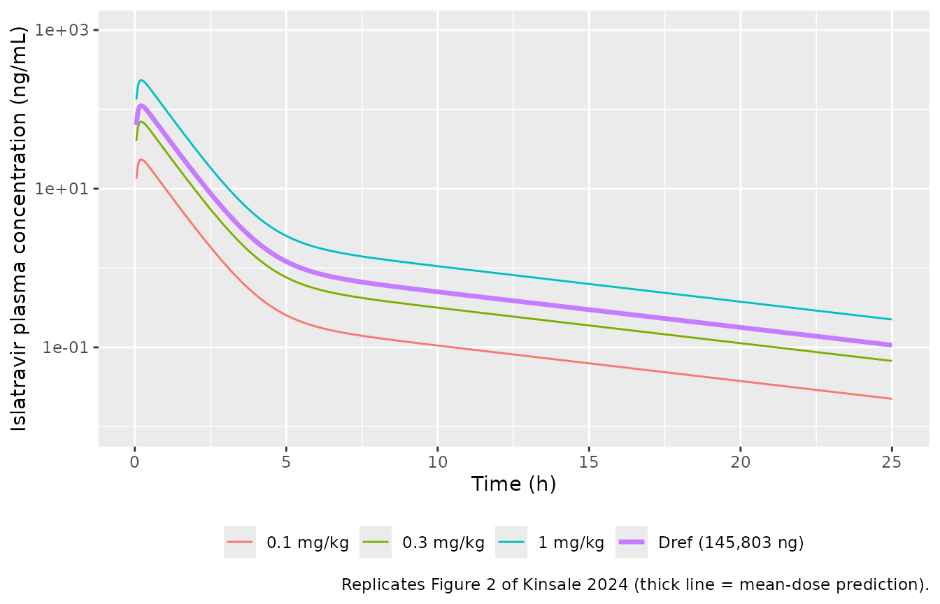
Figure 2’s predicted curve is near 100 ng/mL at the first sample, falls to about 1 ng/mL at 6 h, and to about 0.1 ng/mL at 24 h. The mean-dose prediction takes the values below.
fig2 <- sim |>
  dplyr::filter(treatment == "Dref (145,803 ng)", time %in% c(0.17, 1, 6, 24)) |>
  dplyr::select(time, Cc)
knitr::kable(fig2, digits = 3,
caption = "Mean-dose prediction at selected times (Figure 2 curve).")| time | Cc |
|---|---|
| 0.17 | 109.483 |
| 1.00 | 48.125 |
| 6.00 | 0.866 |
| 24.00 | 0.118 |
# Figure 2 read on its log axis: about 0.8-0.9 ng/mL at 6 h and 0.1 ng/mL at 24 h.
c6 <- fig2$Cc[fig2$time == 6]
c24 <- fig2$Cc[fig2$time == 24]
stopifnot(c6 > 0.6, c6 < 1.2, c24 > 0.07, c24 < 0.15)
PKNCA validation
Kinsale 2024 computed a sparse (naive-pooled) NCA per dose level with
the linear-up / log-down trapezoidal rule on the 0.17-24 h grid (Section
2.5). The typical-value profiles are therefore evaluated on that same
grid. At 0.1 mg/kg the 24 h samples were not quantifiable (Section 3.1),
so the 24 h point is dropped for that dose and its AUClast
ends at 6 h, as in the paper.
# The paper's sampling times plus the pre-dose time zero (pre-dose samples
# were all BLQ, Section 2.3; the simulated Cc at time zero is 0).
nca_times <- c(0, paper_grid)
sim_nca <- sim |>
  dplyr::filter(!is.na(Cc)) |>
  dplyr::filter(
    treatment != "Dref (145,803 ng)",
    time %in% nca_times,
    !(treatment == "0.1 mg/kg" & time == 24)
  ) |>
  dplyr::select(id, time, Cc, treatment) |>
  dplyr::arrange(id, time)
stopifnot(
  nrow(sim_nca) == 3L * length(nca_times) - 1L,
  all(sim_nca$Cc[sim_nca$time == 0] == 0)
)

dose_df <- groups |>
  dplyr::filter(treatment != "Dref (145,803 ng)") |>
  dplyr::mutate(time = 0)

conc_obj <- PKNCA::PKNCAconc(sim_nca, Cc ~ time | treatment + id,
                             concu = "ng/mL", timeu = "h")
dose_obj <- PKNCA::PKNCAdose(dose_df, amt ~ time | treatment + id, doseu = "mg")
intervals <- data.frame(start = 0, end = Inf, cmax = TRUE, tmax = TRUE,
                        auclast = TRUE)

nca_res <- PKNCA::pk.nca(
  PKNCA::PKNCAdata(conc_obj, dose_obj, intervals = intervals,
                   options = list(auc.method = "lin up/log down"))
)
Comparison against published NCA
Published values are from Kinsale 2024 Section 3.1 (plasma ISL;
Tmax 10 min at 0.1 and 1 mg/kg and 30 min at 0.3
mg/kg).
published <- tibble::tribble(
  ~treatment, ~cmax, ~tmax, ~auclast,
  "0.1 mg/kg", 22.6, 0.17, 16.2,
  "0.3 mg/kg", 44.7, 0.5, 54.8,
  "1 mg/kg", 201.3, 0.17, 229.6
)

cmp <- nlmixr2lib::ncaComparisonTable(
  simulated = nca_res,
  reference = published,
  by = "treatment",
  units = c(cmax = "ng/mL", tmax = "h", auclast = "h*ng/mL"),
  tolerance_pct = 20
)
knitr::kable(
  cmp,
  caption = paste(
    "Typical-value NCA vs. published sparse NCA (Kinsale 2024 Section 3.1).",
    "* differs from reference by >20%."
  )
)| NCA parameter | treatment | Reference | Simulated | % diff |
|---|---|---|---|---|
| Cmax (ng/mL) | 0.1 mg/kg | 22.6 | 23.1 | +2.0% |
| Cmax (ng/mL) | 0.3 mg/kg | 44.7 | 69.2 | +54.7%* |
| Cmax (ng/mL) | 1 mg/kg | 201 | 231 | +14.5% |
| Tmax (h) | 0.1 mg/kg | 0.17 | 0.17 | +0.0% |
| Tmax (h) | 0.3 mg/kg | 0.5 | 0.17 | -66.0%* |
| Tmax (h) | 1 mg/kg | 0.17 | 0.17 | +0.0% |
| AUClast (h*ng/mL) | 0.1 mg/kg | 16.2 | 25.1 | +54.7%* |
| AUClast (h*ng/mL) | 0.3 mg/kg | 54.8 | 79.5 | +45.0%* |
| AUClast (h*ng/mL) | 1 mg/kg | 230 | 265 | +15.3% |
sim_wide <- as.data.frame(nca_res$result) |>
  dplyr::filter(PPTESTCD %in% c("cmax", "auclast")) |>
  dplyr::select(treatment, PPTESTCD, PPORRES) |>
  tidyr::pivot_wider(names_from = PPTESTCD, values_from = PPORRES) |>
  dplyr::left_join(
    dplyr::rename(published, cmax_pub = cmax, auclast_pub = auclast),
    by = "treatment"
  ) |>
  dplyr::mutate(
    cmax_ratio = cmax / cmax_pub,
    auclast_ratio = auclast / auclast_pub
  )

knitr::kable(
  sim_wide |>
    dplyr::select(treatment, cmax_ratio, auclast_ratio) |>
    dplyr::rename(
      "Dose level" = treatment,
      "Cmax ratio (model / published)" = cmax_ratio,
      "AUClast ratio (model / published)" = auclast_ratio
    ),
  digits = 2
)| Dose level | Cmax ratio (model / published) | AUClast ratio (model / published) |
|---|---|---|
| 0.1 mg/kg | 1.02 | 1.55 |
| 0.3 mg/kg | 1.55 | 1.45 |
| 1 mg/kg | 1.15 | 1.15 |
# The model is dose proportional; the published AUClast rises more than
# proportionally (slope 1.15). The model sits at the high end at 0.1 mg/kg and
# closest at 1 mg/kg. Every ratio stays within a factor of two of the paper.
stopifnot(
  all(sim_wide$cmax_ratio > 0.5 & sim_wide$cmax_ratio < 2),
  all(sim_wide$auclast_ratio > 0.5 & sim_wide$auclast_ratio < 2)
)
At 1 mg/kg the typical-value Cmax and
AUClast are within 20% of the published values, and the
low-dose Cmax agrees closely. Two discrepancies exceed 20%,
and both come from the published model and data rather than from
transcription:
-
AUClastat 0.1 and 0.3 mg/kg is overpredicted. The pooled fit produced one curve for all three doses, and scaling that curve by dose / Dref is the paper’s own UIR assumption (Section 2.6). The observedAUClast, however, rose more than proportionally with dose (log-log slope 1.15, Section 3.1). A dose-proportional model anchored near the mean dose therefore overpredicts the lower doses. The authors note that their diagnostics give the “best prediction for doses 0.3 mg/kg and higher”, and that low-dose concentrations near the limit of quantification inflated the residual error. -
CmaxandTmaxat 0.3 mg/kg. The observed mid-dose peak fell at 30 min, against 10 min for the other two doses. The authors attribute this to “random variability due to sparse sampling methods” with three destructively sampled rats per time point (Discussion). The typical-value model, with Ka = 12.23 1/h, peaks before 30 min at every dose.
Implant illustration: zero-order systemic input
Section 3.3 reports a deconvolved mean in vivo absorption rate of
0.072 +/- 0.024 mg/day (ISL-only 0.084, ISL-plus 0.061 mg/day) for the
reservoir-style implant over 0-154 days, and Table 1 shows that a
zero-order model describes the cumulative absorbed mass well (mean
r2 0.946). The deconvolution used the UIR as the systemic
disposition, so the implant input enters central directly.
The illustration below applies these mean rates as constant-rate inputs.
It is not a fit to the implant data (the individual implant PK was
published separately and is not reproduced here). At steady state the
plasma concentration is rate / CL.
rates <- tibble::tibble(
  id = 1:3,
  treatment = c("Overall mean 0.072 mg/day", "ISL-only 0.084 mg/day",
                "ISL-plus 0.061 mg/day"),
  rate_mg_day = c(0.072, 0.084, 0.061)
)
t_end_h <- 154 * 24

ev_implant <- dplyr::bind_rows(lapply(seq_len(nrow(rates)), function(i) {
  ev <- rxode2::et(
    amt = rates$rate_mg_day[i] * 154, rate = rates$rate_mg_day[i] / 24,
    cmt = "central"
  ) |>
    rxode2::et(seq(0, t_end_h, by = 24), cmt = "central") |>
    as.data.frame()
  ev$id <- rates$id[i]
  ev$treatment <- rates$treatment[i]
  ev
}))

sim_implant <- rxode2::rxSolve(mod, events = ev_implant, keep = "treatment") |>
  as.data.frame()
#> Warning: multi-subject simulation without without 'omega'

ggplot2::ggplot(sim_implant, ggplot2::aes(time / 24, Cc, colour = treatment)) +
  ggplot2::geom_line() +
  ggplot2::labs(x = "Time after implantation (day)",
                y = "Islatravir plasma concentration (ng/mL)", colour = NULL,
                caption = "Illustration: constant-rate input at the Section 3.3 mean absorption rates.") +
  ggplot2::theme(legend.position = "bottom")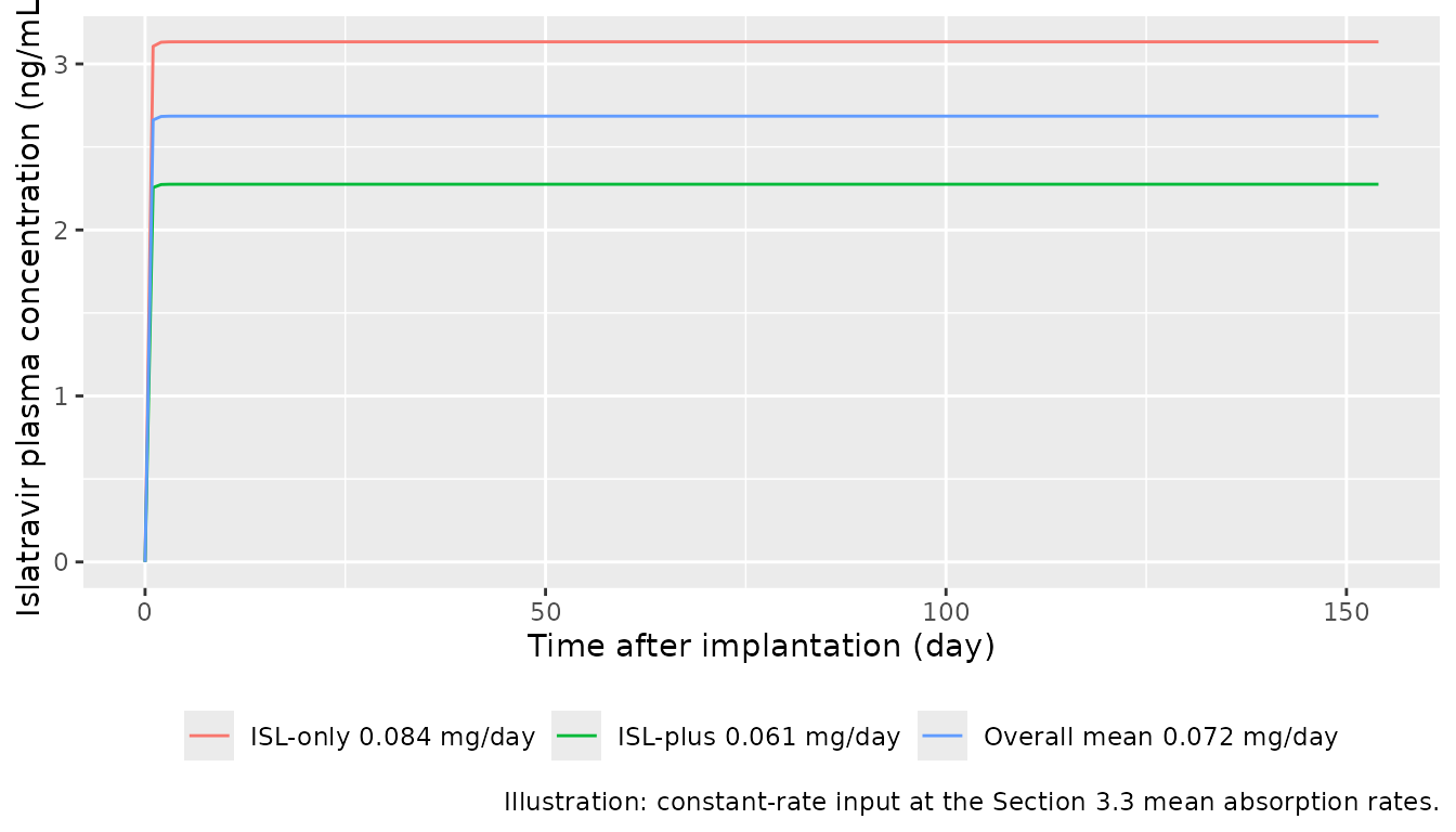
css <- sim_implant |>
  dplyr::filter(time == 100 * 24) |>
  dplyr::select(treatment, Cc) |>
  dplyr::mutate(`Rate / CL (ng/mL)` = rates$rate_mg_day / 24 / p$cl[1] * 1000)
knitr::kable(css, digits = 3, caption = "Plateau concentration at day 100.")| treatment | Cc | Rate / CL (ng/mL) |
|---|---|---|
| Overall mean 0.072 mg/day | 2.686 | 2.686 |
| ISL-only 0.084 mg/day | 3.133 | 3.133 |
| ISL-plus 0.061 mg/day | 2.275 | 2.275 |
Assumptions and deviations
-
Naive-pooled fit, dose-proportional encoding. The
published fit reports the macro-constants A and B in ng/mL for one
pooled curve across all three doses (Figure 2). The model writes the
paper’s UIR (A / Dref, B / Dref, with Dref = 145,803 ng from Section
2.6) as
vcandk21, so a dose of Dref reproduces the fitted curve and other doses scale proportionally. This is the assumption the paper itself makes when it uses the UIR for deconvolution, and it is supported by the dose-proportionality slopes in Section 3.1.lvcandlk21are therefore derived values; the source-trace table gives their derivation. - Macro-constant reading with first-order absorption. The model treats A and B as coefficients of the impulse (bolus) response, with first-order absorption convolved into it. This is how Section 2.6 uses them (A / dose = UIR) and is consistent with the stripping-dose macro parameterisation of Phoenix NLME. If A and B were instead the coefficients of the extravascular curve itself, A would be about 10% smaller (factor (Ka - alpha) / Ka = 0.90) and B about 1% smaller. The two readings cannot be distinguished at the resolution of Figure 2.
- Final-model estimates. Values come from the ‘Final’ column of Supplementary Table S1 (model 6, ‘Base Model no Outlier’), which matches the rounded Figure 2 inset. Section 3.2 prints A1 = 9.8 x 10⁻⁴ ng/mL/ng; the Table S1 value gives 9.71 x 10⁻⁴ (see the UIR section).
-
Residual error. The 76% residual error of the
Phoenix multiplicative error model (Section 3.2; Table S1, model 6) is
encoded as proportional error,
propSd = 0.76. - No IIV. The naive-pooled algorithm estimates no between-animal variability, so the model has no etas; this reflects the analysis design, not an unreported variance.
- Body weight. Doses are mg/kg. The vignette uses the mean body weight (0.307 kg) to convert to mg; the model has no weight covariate because the paper’s fit has none.
- Not modelled. Intracellular ISL-triphosphate in PBMCs was analysed by NCA only. The deconvolution and the four release-kinetic regressions (Table 1) produce rates and goodness-of-fit statistics rather than model parameters (zero-order and Ritger-Peppas rate constants are not reported). The implant appears only as the constant-rate illustration above.
- Errata. A literature search on 2026-10-29 (Europe PMC) found no erratum or correction for this article.