Sapanisertib concentration-QTc and concentration-RR (Patel 2020)
Source:vignettes/articles/Patel_2020_sapanisertib.Rmd
Patel_2020_sapanisertib.RmdModel and source
- Citation: Patel C, Goel S, Patel MR, Rangachari L, Wilbur JD, Shou Y, Venkatakrishnan K, Lockhart AC. (2020). Phase 1 Study to Evaluate the Effect of the Investigational Anticancer Agent Sapanisertib on the QTc Interval in Patients With Advanced Solid Tumors. Clinical Pharmacology in Drug Development 9(7):876-888. doi:10.1002/cpdd.808.
- Article: https://doi.org/10.1002/cpdd.808
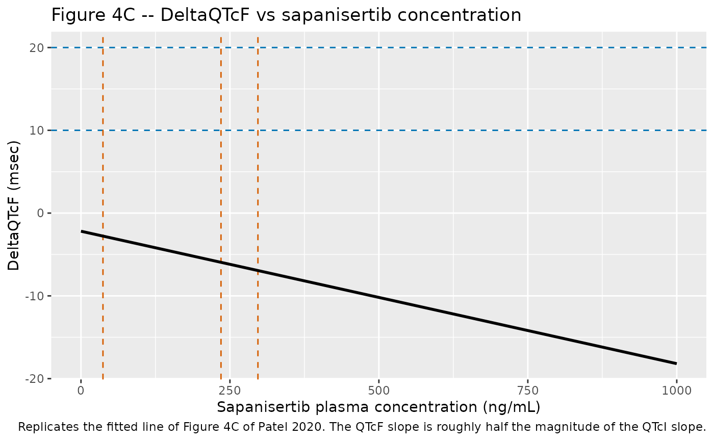
Patel et al. (2020) report a dedicated QTc (DQT) study of the mTORC1/2 inhibitor sapanisertib (MLN0128 / INK128 / TAK-228) in 44 patients with advanced solid tumors, each given a single supratherapeutic 40 mg oral dose with time-matched day -1 baseline Holter electrocardiograms. Three linear mixed-effects concentration-effect models were fitted independently, one per electrocardiographic endpoint, and are packaged here as three model files sharing one vignette:
| Model file | Endpoint | Source panel |
|---|---|---|
Patel_2020_sapanisertib_QTcI |
change from time-matched baseline in the individually rate-corrected
QT interval (QTcI, msec) |
Figure 4A |
Patel_2020_sapanisertib_QTcF |
change from time-matched baseline in the Fridericia-corrected QT
interval (QTcF, msec) |
Figure 4C |
Patel_2020_sapanisertib_RR |
change from time-matched baseline in the RR interval
(d_rr, msec) |
Supplementary Figure S2 |
All three share the identical algebraic structure
and all three are PD-only: the source paper fits no
population PK model, so sapanisertib plasma concentration enters as the
time-varying covariate CP_SAPANISERTIB_NGML (ng/mL) rather
than being computed from an internal compartment system.
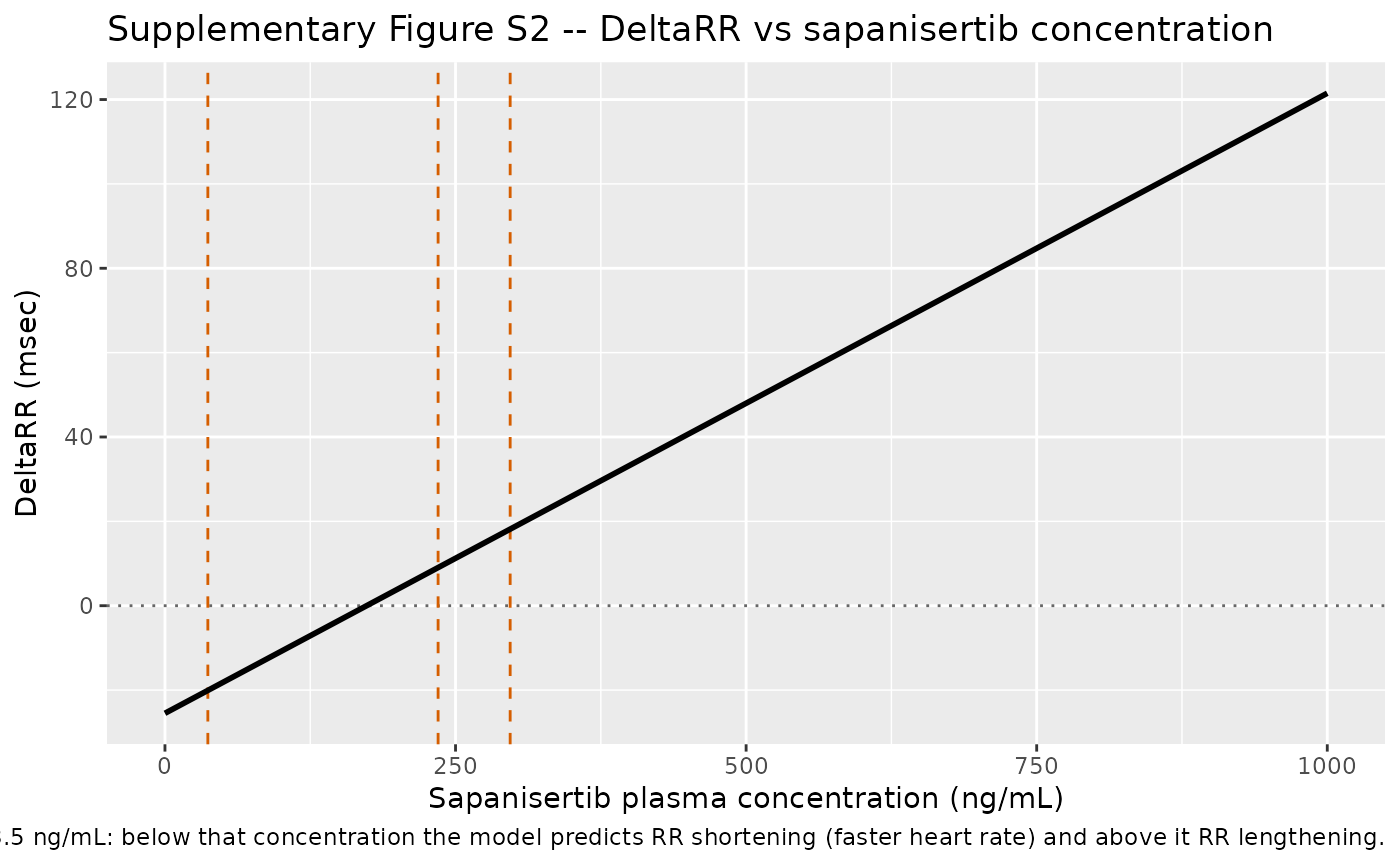
The paper’s central finding is negative, and the sign structure carries it. Both QTc slopes are negative – rising sapanisertib concentration is associated with QTc shortening, not prolongation – while the RR slope is positive (RR lengthening, i.e. heart-rate slowing). A user who assumes a common sign convention across the three files will misread one of them.
Population
Forty-four adults with a radiographically or clinically evaluable advanced solid tumor were enrolled at 5 United States centers (NCT02197572) and received the single 40 mg dose. Median age was 59.5 years (range 22-79), 16 of 44 (36%) were male, and median weight was 70.6 kg (range 49-122). Reported race was White in 30 (68%), Black in 9 (20%) and not reported in 5 (11%). Disease stage was IV or higher in 34 of 44 (77%) and 42 of 44 (95%) had received prior antineoplastic therapy; ECOG performance status was 0 in 13 (30%), 1 in 30 (68%) and 2 in 1 (2%) (Patel 2020 Table 1).
Two features of the cohort matter for interpreting the models. First, the eligibility criteria excluded patients with baseline QTcF above 430 msec (men) or 450 msec (women), congenital long QT syndrome, diabetes mellitus, gastrointestinal disease, or significant active cardiovascular or pulmonary disease (Patel 2020 Supplemental Methods, “Patients”), so the cohort is pre-selected against QT-vulnerable patients. Second, the analysis populations differ: all 44 patients contributed to the concentration-effect analysis these model files encode, whereas the separate repeated-measures least-squares-mean analysis (Patel 2020 Table 2 and Supplementary Table S1) used only the 32 patients with a complete day -1 / day 1 Holter series. The models below must not be gated against Table 2 or Table S1.
The same information is available programmatically via each model’s
population metadata,
e.g. readModelDb("Patel_2020_sapanisertib_QTcI")()$population.
Source trace
Every value in every ini() block comes from a
regression-summary table printed inside a figure panel.
Those in-panel tables carry full printed-value authority – they are
printed parameter tables, not digitised or curve-fitted values – but
they are invisible to plain-text extraction of the PDF (including
pdftotext) because Figures 4 and S2 are raster images. They
were recovered with pdftoppm -r 400 -f 10 on the article
PDF (Figures 4A and 4C, journal page 885) and by unzipping
cpdd808-sup-0001-suppmat.docx and rendering
word/media/image4.png (Figure S2).
| Model | Parameter | Value | Source location (printed Estimate / SE / df / t / P / 95% bootstrap CI) |
|---|---|---|---|
| QTcI | e0 |
-0.304 msec | Fig 4A panel table, Intercept: -0.304 / 1.755 / 409 / -0.173 / 0.863 / (-3.757, 3.177) |
| QTcI | slope |
-0.033 msec per ng/mL | Fig 4A panel table, Slope: -0.033 / 0.011 / 409 / -3.137 / 0.002 / (-0.060, -0.013) |
| QTcI | addSd |
fixed(0) |
Not reported in source – typical-value model (see Errata) |
| QTcF | e0 |
-2.189 msec | Fig 4C panel table, Intercept: -2.189 / 1.137 / 440 / -1.926 / 0.055 / (-4.618, 0.220) |
| QTcF | slope |
-0.016 msec per ng/mL | Fig 4C panel table, Slope: -0.016 / 0.006 / 440 / -2.446 / 0.015 / (-0.033, -0.003) |
| QTcF | addSd |
fixed(0) |
Not reported in source – typical-value model (see Errata) |
| RR | e0 |
-25.504 msec | Fig S2 panel table, Intercept: -25.504 / 9.453 / 470 / -2.698 / 0.007 / (-44.154, -7.851) |
| RR | slope |
+0.147 msec per ng/mL | Fig S2 panel table, Slope: 0.147 / 0.034 / 470 / 4.278 / 0.000 / (0.082, 0.242) |
| RR | addSd |
fixed(0) |
Not reported in source – typical-value model (see Errata) |
| All | CP_SAPANISERTIB_NGML |
ng/mL, time-varying | Patel 2020 Figures 4A / 4C / S2 x-axis, “Concentration (ng mL-1)” |
| All | Equation form | linear, intercept + slope | Patel 2020 Results, “Relationship of Sapanisertib Concentration and QTc” / “… and Heart Rate” |
Verification of the printed panel tables
Because the six estimates were read off raster images, each panel
table was checked for internal arithmetic consistency before being
trusted. The recomputed two-sided P-value from each printed
(t, df) pair must reproduce the printed P-value, and each
printed bootstrap confidence interval must contain its own point
estimate.
panels <- tibble::tribble(
  ~model,  ~parameter,   ~est,     ~se,    ~df, ~t_print, ~p_print, ~ci_lo,   ~ci_hi,
  "QTcI",  "Intercept",  -0.304,   1.755,  409, -0.173,   0.863,    -3.757,    3.177,
  "QTcI",  "Slope",      -0.033,   0.011,  409, -3.137,   0.002,    -0.060,   -0.013,
  "QTcF",  "Intercept",  -2.189,   1.137,  440, -1.926,   0.055,    -4.618,    0.220,
  "QTcF",  "Slope",      -0.016,   0.006,  440, -2.446,   0.015,    -0.033,   -0.003,
  "RR",    "Intercept", -25.504,   9.453,  470, -2.698,   0.007,   -44.154,   -7.851,
  "RR",    "Slope",       0.147,   0.034,  470,  4.278,   0.000,     0.082,    0.242
) |>
  dplyr::mutate(
    p_recomputed = 2 * stats::pt(-abs(t_print), df),
    p_agrees     = abs(p_recomputed - p_print) < 5e-4,
    ci_contains  = est >= ci_lo & est <= ci_hi
  )

panels |>
  dplyr::transmute(
    Model                 = model,
    Parameter             = parameter,
    Estimate              = est,
    SE                    = se,
    df                    = df,
    `t (printed)`         = t_print,
    `P (printed)`         = p_print,
    `P from (t, df)`      = signif(p_recomputed, 3),
    `P agrees`            = p_agrees,
    `CI contains estimate` = ci_contains
  ) |>
  knitr::kable(
    caption = paste(
      "Internal consistency of the six printed in-panel regression summaries.",
      "Every P-value reproduces from its own t-value and residual degrees of",
      "freedom, and every bootstrap CI contains its point estimate."
    )
)| Model | Parameter | Estimate | SE | df | t (printed) | P (printed) | P from (t, df) | P agrees | CI contains estimate |
|---|---|---|---|---|---|---|---|---|---|
| QTcI | Intercept | -0.304 | 1.755 | 409 | -0.173 | 0.863 | 8.63e-01 | TRUE | TRUE |
| QTcI | Slope | -0.033 | 0.011 | 409 | -3.137 | 0.002 | 1.83e-03 | TRUE | TRUE |
| QTcF | Intercept | -2.189 | 1.137 | 440 | -1.926 | 0.055 | 5.47e-02 | TRUE | TRUE |
| QTcF | Slope | -0.016 | 0.006 | 440 | -2.446 | 0.015 | 1.48e-02 | TRUE | TRUE |
| RR | Intercept | -25.504 | 9.453 | 470 | -2.698 | 0.007 | 7.23e-03 | TRUE | TRUE |
| RR | Slope | 0.147 | 0.034 | 470 | 4.278 | 0.000 | 2.29e-05 | TRUE | TRUE |
Independent corroboration of the two QTc lines
Table 4 of the paper tabulates model-predicted DeltaQTcI
and DeltaQTcF at three geometric-mean Cmax anchors – 36.9
ng/mL (4 mg once daily), 235 ng/mL (30 mg once weekly) and 297 ng/mL
(the 40 mg dose of this study). Three points
over-determine a two-parameter line, so Table 4 can be
inverted and compared against the Figure 4 panel tables. This is a
genuinely independent printed source: it is set as text in the article
body, not drawn inside a figure.
table4 <- tibble::tribble(
  ~dose_mg, ~cmax_ngml, ~dQTcI,  ~dQTcF,
  4,          36.9,      -1.538,  -2.762,
  30,        235.0,      -8.159,  -5.837,
  40,        297.0,     -10.231,  -6.800
)

invert_line <- function(y) {
  fit <- stats::lm(y ~ table4$cmax_ngml)
  c(
    intercept = unname(stats::coef(fit)[1]),
    slope     = unname(stats::coef(fit)[2]),
    r_squared = summary(fit)$r.squared
  )
}

# Table 4 itself prints only three decimals, so the inversion inherits that
# granularity. Enumerating the 27 corner perturbations of +/-0.0005 on the
# three anchors bounds how far the inverted intercept and slope can move.
invert_band <- function(y) {
  corners <- expand.grid(a = c(-1, 0, 1), b = c(-1, 0, 1), c = c(-1, 0, 1))
  co <- t(apply(corners, 1, function(r) {
    stats::coef(stats::lm((y + 5e-4 * as.numeric(r)) ~ table4$cmax_ngml))
  }))
  c(
    intercept_lo = min(co[, 1]), intercept_hi = max(co[, 1]),
    slope_lo     = min(co[, 2]), slope_hi     = max(co[, 2])
  )
}

inverted <- dplyr::bind_cols(
  tibble::tibble(model = c("QTcI", "QTcF")),
  dplyr::bind_rows(
    as.data.frame(t(invert_line(table4$dQTcI))),
    as.data.frame(t(invert_line(table4$dQTcF)))
  ),
  dplyr::bind_rows(
    as.data.frame(t(invert_band(table4$dQTcI))),
    as.data.frame(t(invert_band(table4$dQTcF)))
  )
) |>
  dplyr::mutate(
    panel_intercept = c(-0.304, -2.189),
    panel_slope     = c(-0.033, -0.016),
    # Two printed sources, each rounded to three decimals, are consistent when
    # their rounding intervals overlap.
    intercept_consistent =
      intercept_lo - 5e-4 <= panel_intercept + 5e-4 &
      intercept_hi + 5e-4 >= panel_intercept - 5e-4,
    slope_consistent =
      slope_lo - 5e-4 <= panel_slope + 5e-4 &
      slope_hi + 5e-4 >= panel_slope - 5e-4
  )

inverted |>
  dplyr::transmute(
    Model                        = model,
    `Intercept (Table 4)`        = round(intercept, 5),
    `Intercept band from Table 4 rounding` =
      paste0("[", round(intercept_lo, 4), ", ", round(intercept_hi, 4), "]"),
    `Intercept (Fig 4 panel)`    = panel_intercept,
    `Slope (Table 4)`            = signif(slope, 6),
    `Slope (Fig 4 panel)`        = panel_slope,
    `R-squared of the 3 anchors` = signif(r_squared, 10)
  ) |>
  knitr::kable(
    caption = paste(
      "Inverting Table 4's three collinear Cmax anchors recovers the Figure 4",
      "panel estimates. Both sources print three decimals, so agreement is",
      "assessed by overlap of the two rounding intervals rather than by exact",
      "equality: the inverted QTcI intercept -0.30475 does not itself round to",
      "the printed -0.304, but Table 4's own rounding admits any intercept in",
      "[-0.3055, -0.3040], which overlaps the panel's [-0.3045, -0.3035]."
    )
)| Model | Intercept (Table 4) | Intercept band from Table 4 rounding | Intercept (Fig 4 panel) | Slope (Table 4) | Slope (Fig 4 panel) | R-squared of the 3 anchors |
|---|---|---|---|---|---|---|
| QTcI | -0.30475 | [-0.3055, -0.304] | -0.304 | -0.0334219 | -0.033 | 1 |
| QTcF | -2.18909 | [-2.1898, -2.1884] | -2.189 | -0.0155242 | -0.016 | 1 |
stopifnot(
  # The three Table 4 anchors are collinear to numerical precision, which is
  # what licenses the inversion at all.
  all(inverted$r_squared > 0.9999999),
  # The two independent printed sources are mutually consistent.
  all(inverted$intercept_consistent),
  all(inverted$slope_consistent),
  # And the point inversion sits within 0.001 of each printed panel value.
  all(abs(inverted$intercept - inverted$panel_intercept) < 1e-3),
  all(abs(inverted$slope - inverted$panel_slope) < 1e-3)
)
A third, sharper check falls out of this. Estimate / SE
computed from the printed three-decimal panel values does
not reproduce the printed t for either
slope (-0.033 / 0.011 = -3.04, printed
-3.137), which on its own could look like a transcription
error. It is not: dividing the unrounded slope recovered from
Table 4 by the printed t recovers a standard error that
rounds back to the printed SE. Both printed numbers are simply rounded
to three decimals, and the two independent sources agree once the
rounding is undone.
se_check <- inverted |>
  dplyr::transmute(
    Model                  = model,
    `Unrounded slope`      = signif(slope, 6),
    `t printed in panel`   = c(-3.137, -2.446),
    `Implied SE`           = signif(slope / c(-3.137, -2.446), 5),
    `Implied SE rounded`   = round(slope / c(-3.137, -2.446), 3),
    `SE printed in panel`  = c(0.011, 0.006),
    `Naive t from printed values` = round(c(-0.033, -0.016) / c(0.011, 0.006), 3)
  )
knitr::kable(
  se_check,
  caption = paste(
    "The standard error implied by the Table-4-derived unrounded slope and the",
    "printed t-value rounds back to the printed SE, so the apparent",
    "Estimate/SE/t inconsistency in the panels is three-decimal rounding.",
    "This cross-checks the slope AND the SE against two independent printed",
    "sources."
  )
)| Model | Unrounded slope | t printed in panel | Implied SE | Implied SE rounded | SE printed in panel | Naive t from printed values |
|---|---|---|---|---|---|---|
| QTcI | -0.0334219 | -3.137 | 0.0106540 | 0.011 | 0.011 | -3.000 |
| QTcF | -0.0155242 | -2.446 | 0.0063468 | 0.006 | 0.006 | -2.667 |
The DeltaRR model has no counterpart to Table 4 – Table
4 covers the two QTc endpoints only – so its verification rests on the
internal Estimate / SE / t / P / CI redundancy shown above. There,
Estimate / SE reproduces the printed t
directly for the intercept (-25.504 / 9.453 = -2.698,
exactly as printed).
Virtual cohort
The paper presents all three models in the concentration domain (Figures 4A, 4C and S2 plot the endpoint against sapanisertib concentration; Table 4 gives point predictions at three concentrations). There is no time-domain model output in the paper, so the primary reproduction below is a concentration grid rather than a simulated time course.
The grid spans 0 to 1000 ng/mL, matching the x-axis extent of all three figure panels; the observed concentration-effect dataset ranged from below the limit of quantification to a maximum individual Cmax of 976 ng/mL (Patel 2020 Supplementary Table S2, Cmax median 317, range 94-976). Because the models are purely algebraic with no time dependence, one observation event per grid point is sufficient – and well under the 200-per-arm cohort cap.
Simulation
Each model returns its change-from-time-matched-baseline endpoint
directly as the observation variable (QTcI,
QTcF, d_rr). No etas are declared – the source
reports no variance components – so zeroRe() is unnecessary
and omega = NA must not be passed.
mod_qtci <- readModelDb("Patel_2020_sapanisertib_QTcI")
mod_qtcf <- readModelDb("Patel_2020_sapanisertib_QTcF")
mod_rr   <- readModelDb("Patel_2020_sapanisertib_RR")

sim_qtci <- rxode2::rxSolve(mod_qtci, events = events, keep = "conc") |>
  as.data.frame()
#> Warning: multi-subject simulation without without 'omega'
sim_qtcf <- rxode2::rxSolve(mod_qtcf, events = events, keep = "conc") |>
  as.data.frame()
#> Warning: multi-subject simulation without without 'omega'
sim_rr <- rxode2::rxSolve(mod_rr, events = events, keep = "conc") |>
  as.data.frame()
#> Warning: multi-subject simulation without without 'omega'

cmax_anchors <- tibble::tibble(
  dose  = c("4 mg", "30 mg", "40 mg"),
  cmax  = c(36.9, 235.0, 297.0)
)
The three slopes must carry the signs the paper reports, and the two QTc endpoints must remain far below the 20-msec threshold the paper treats as clinically relevant for an oncology DQT study, across the whole observed concentration range.
stopifnot(
  # Both QTc endpoints decrease with concentration (the paper's negative finding).
  all(diff(sim_qtci$QTcI) < 0),
  all(diff(sim_qtcf$QTcF) < 0),
  # The RR interval lengthens with concentration (heart-rate slowing).
  all(diff(sim_rr$d_rr) > 0),
  # No QTc prolongation anywhere in the observed range, let alone 10 or 20 msec.
  max(sim_qtci$QTcI) <= 0,
  max(sim_qtcf$QTcF) <= 0
)
Replicate published figures
Figure 4A – DeltaQTcI versus sapanisertib
concentration
ggplot(sim_qtci, aes(conc, QTcI)) +
  geom_hline(yintercept = c(10, 20), linetype = "dashed",
             colour = "#0072B2") +
  geom_vline(data = cmax_anchors, aes(xintercept = cmax),
             linetype = "dashed", colour = "#D55E00") +
  geom_line(linewidth = 1) +
  labs(
    x = "Sapanisertib plasma concentration (ng/mL)",
    y = "DeltaQTcI (msec)",
    title = "Figure 4A -- DeltaQTcI vs sapanisertib concentration",
    caption = paste(
      "Replicates the fitted line of Figure 4A of Patel 2020.",
      "Vertical lines: geometric-mean Cmax for 4, 30 and 40 mg.",
      "Horizontal lines: the 10 and 20 msec reference levels."
    )
  )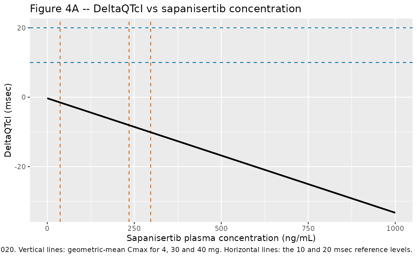
Figure 4C – DeltaQTcF versus sapanisertib
concentration
ggplot(sim_qtcf, aes(conc, QTcF)) +
  geom_hline(yintercept = c(10, 20), linetype = "dashed",
             colour = "#0072B2") +
  geom_vline(data = cmax_anchors, aes(xintercept = cmax),
             linetype = "dashed", colour = "#D55E00") +
  geom_line(linewidth = 1) +
  labs(
    x = "Sapanisertib plasma concentration (ng/mL)",
    y = "DeltaQTcF (msec)",
    title = "Figure 4C -- DeltaQTcF vs sapanisertib concentration",
    caption = paste(
      "Replicates the fitted line of Figure 4C of Patel 2020.",
      "The QTcF slope is roughly half the magnitude of the QTcI slope."
    )
  )
Supplementary Figure S2 – DeltaRR versus sapanisertib
concentration
zero_cross <- -readModelDb("Patel_2020_sapanisertib_RR")()$theta[["e0"]] /
  readModelDb("Patel_2020_sapanisertib_RR")()$theta[["slope"]]

ggplot(sim_rr, aes(conc, d_rr)) +
  geom_hline(yintercept = 0, linetype = "dotted", colour = "grey40") +
  geom_vline(data = cmax_anchors, aes(xintercept = cmax),
             linetype = "dashed", colour = "#D55E00") +
  geom_line(linewidth = 1) +
  labs(
    x = "Sapanisertib plasma concentration (ng/mL)",
    y = "DeltaRR (msec)",
    title = "Supplementary Figure S2 -- DeltaRR vs sapanisertib concentration",
    caption = paste0(
      "Replicates the fitted line of Figure S2 of Patel 2020. ",
      "The line crosses zero at ", round(zero_cross, 1), " ng/mL: below that ",
      "concentration the model predicts RR shortening (faster heart rate) ",
      "and above it RR lengthening."
    )
  )
Validation gate: reproducing Table 4
Table 4 is a zero-parameter gate on the two QTc
models: it contains six model-predicted values that the packaged models
must reproduce with no fitting, no seed and no free choices at all. The
models ship the printed three-decimal panel estimates, so that
every number in ini() is a number printed in the paper;
that rounding is the only source of disagreement.
predict_endpoint <- function(mod, conc) {
  ev <- tibble::tibble(
    id                   = seq_along(conc),
    CP_SAPANISERTIB_NGML = conc,
    time                 = 0,
    evid                 = 0,
    amt                  = 0,
    cmt                  = NA_character_
  )
  as.data.frame(rxode2::rxSolve(mod, events = ev))
}

gate <- table4 |>
  dplyr::mutate(
    model_dQTcI = predict_endpoint(mod_qtci, cmax_ngml)$QTcI,
    model_dQTcF = predict_endpoint(mod_qtcf, cmax_ngml)$QTcF,
    diff_dQTcI  = model_dQTcI - dQTcI,
    diff_dQTcF  = model_dQTcF - dQTcF
  )
#> Warning: There were 2 warnings in `dplyr::mutate()`.
#> The first warning was:
#> ℹ In argument: `model_dQTcI = predict_endpoint(mod_qtci, cmax_ngml)$QTcI`.
#> Caused by warning:
#> ! multi-subject simulation without without 'omega'
#> ℹ Run `dplyr::last_dplyr_warnings()` to see the 1 remaining warning.

gate |>
  dplyr::transmute(
    `Dose`                       = paste(dose_mg, "mg"),
    `Geometric mean Cmax (ng/mL)` = cmax_ngml,
    `Paper DeltaQTcI (msec)`     = dQTcI,
    `Model DeltaQTcI (msec)`     = round(model_dQTcI, 3),
    `QTcI diff`                  = round(diff_dQTcI, 3),
    `Paper DeltaQTcF (msec)`     = dQTcF,
    `Model DeltaQTcF (msec)`     = round(model_dQTcF, 3),
    `QTcF diff`                  = round(diff_dQTcF, 3)
  ) |>
  knitr::kable(
    caption = paste(
      "Zero-parameter validation against Patel 2020 Table 4. Model values use",
      "the printed three-decimal Figure 4 panel estimates; all six agree with",
      "the paper to within 0.15 msec, which is entirely slope rounding."
    )
)| Dose | Geometric mean Cmax (ng/mL) | Paper DeltaQTcI (msec) | Model DeltaQTcI (msec) | QTcI diff | Paper DeltaQTcF (msec) | Model DeltaQTcF (msec) | QTcF diff |
|---|---|---|---|---|---|---|---|
| 4 mg | 36.9 | -1.538 | -1.522 | 0.016 | -2.762 | -2.779 | -0.017 |
| 30 mg | 235.0 | -8.159 | -8.059 | 0.100 | -5.837 | -5.949 | -0.112 |
| 40 mg | 297.0 | -10.231 | -10.105 | 0.126 | -6.800 | -6.941 | -0.141 |
stopifnot(
  # Deterministic comparison -- no random draws on either side -- so a tight
  # bound on every one of the six values is the correct assertion.
  all(abs(gate$diff_dQTcI) < 0.15),
  all(abs(gate$diff_dQTcF) < 0.15)
)
Using the unrounded slopes and intercepts recovered from Table 4
instead of the printed three-decimal values collapses the residual to
numerical noise, which confirms that the 0.15 msec offset above is
rounding and nothing else. Users who need to reproduce Table 4
digit-for-digit should override ini() with the unrounded
values.
exact <- gate |>
  dplyr::mutate(
    exact_dQTcI = inverted$intercept[1] + inverted$slope[1] * cmax_ngml,
    exact_dQTcF = inverted$intercept[2] + inverted$slope[2] * cmax_ngml,
    ediff_dQTcI = exact_dQTcI - dQTcI,
    ediff_dQTcF = exact_dQTcF - dQTcF
  )

exact |>
  dplyr::transmute(
    `Dose`                        = paste(dose_mg, "mg"),
    `Paper DeltaQTcI (msec)`      = dQTcI,
    `Unrounded model DeltaQTcI`   = round(exact_dQTcI, 5),
    `QTcI diff`                   = signif(ediff_dQTcI, 3),
    `Paper DeltaQTcF (msec)`      = dQTcF,
    `Unrounded model DeltaQTcF`   = round(exact_dQTcF, 5),
    `QTcF diff`                   = signif(ediff_dQTcF, 3)
  ) |>
  knitr::kable(
    caption = paste(
      "The same gate using the unrounded intercept and slope back-solved from",
      "Table 4. Residuals fall to below 0.001 msec, isolating the rounding."
    )
)| Dose | Paper DeltaQTcI (msec) | Unrounded model DeltaQTcI | QTcI diff | Paper DeltaQTcF (msec) | Unrounded model DeltaQTcF | QTcF diff |
|---|---|---|---|---|---|---|
| 4 mg | -1.538 | -1.53802 | -2.17e-05 | -2.762 | -2.76193 | 6.74e-05 |
| 30 mg | -8.159 | -8.15891 | 9.11e-05 | -5.837 | -5.83728 | -2.83e-04 |
| 40 mg | -10.231 | -10.23107 | -6.94e-05 | -6.800 | -6.79978 | 2.15e-04 |
Illustrative time course
The three packaged models are algebraic in concentration; driving them over time requires an external sapanisertib concentration trajectory, which this paper does not supply as a model. The chunk below builds a purely illustrative one-compartment oral trajectory in order to demonstrate the time-varying-covariate usage pattern. It is anchored on three numbers printed in Supplementary Table S2 for the study’s 40 mg dose – geometric mean Cmax 297 ng/mL, median Tmax 1.52 h and geometric mean AUC-infinity 2480 ng*h/mL – which exactly determine the three Bateman parameters.
This reconstruction is not part of any model file and is not a fit reported by the paper. It also carries a diagnostic message: matching Cmax, Tmax and AUC-infinity simultaneously forces an apparent terminal half-life of about 4.6 h, roughly half the 9.06 h geometric-mean terminal half-life the paper reports. A one-compartment form cannot satisfy both the observed Cmax/AUC ratio and the observed terminal slope, which is direct evidence of multi-compartment disposition that the paper’s non-compartmental analysis leaves unmodelled. Anyone needing a quantitative sapanisertib PK driver should obtain a genuine popPK model rather than use this illustration.
dose_mg <- 40
cl_f    <- dose_mg * 1000 / 2480 # L/h, from AUCinf = Dose / (CL/F)
tmax_h  <- 1.52
cmax    <- 297

# For a one-compartment oral model, Cmax = (Dose / V) * exp(-kel * Tmax), which
# with CL/F = V * kel determines V, then kel, then ka via the Tmax identity.
v_f <- stats::uniroot(
  function(v) v - (dose_mg * 1000 / cmax) * exp(-tmax_h * cl_f / v),
  interval = c(100, 1000)
)$root
kel <- cl_f / v_f
ka <- stats::uniroot(
  function(ka) log(ka / kel) / (ka - kel) - tmax_h,
  interval = c(kel * 1.0001, 500)
)$root

bateman <- function(t) {
  dose_mg * ka / (v_f * (ka - kel)) * (exp(-kel * t) - exp(-ka * t)) * 1000
}

c(
  `CL/F (L/h)`               = round(cl_f, 2),
  `V/F (L)`                  = round(v_f, 1),
  `ka (1/h)`                 = round(ka, 3),
  `implied t1/2 (h)`         = round(log(2) / kel, 2),
  `reproduced Cmax (ng/mL)`  = round(bateman(tmax_h), 1),
  `reproduced AUCinf`        = round(dose_mg / cl_f * 1000, 0)
)
#>              CL/F (L/h)                 V/F (L)                ka (1/h)
#>                  16.130                 107.100                   1.773
#>        implied t1/2 (h) reproduced Cmax (ng/mL)       reproduced AUCinf
#>                   4.600                 297.000                2480.000

stopifnot(
  # The reconstruction hits its three printed anchors by construction; this
  # asserts the numerics converged, not anything about the paper.
  abs(bateman(tmax_h) - cmax) < 0.01,
  abs(dose_mg / cl_f * 1000 - 2480) < 1
)
tc_events <- tibble::tibble(
  time = c(seq(0, 12, by = 0.1), seq(12.5, 48, by = 0.5))
) |>
  dplyr::mutate(
    id                   = 1L,
    CP_SAPANISERTIB_NGML = bateman(time),
    evid                 = 0,
    amt                  = 0,
    cmt                  = NA_character_
  )

tc <- dplyr::bind_rows(
  as.data.frame(rxode2::rxSolve(mod_qtci, events = tc_events)) |>
    dplyr::transmute(time, value = QTcI, endpoint = "DeltaQTcI"),
  as.data.frame(rxode2::rxSolve(mod_qtcf, events = tc_events)) |>
    dplyr::transmute(time, value = QTcF, endpoint = "DeltaQTcF"),
  as.data.frame(rxode2::rxSolve(mod_rr, events = tc_events)) |>
    dplyr::transmute(time, value = d_rr, endpoint = "DeltaRR")
)

ggplot(tc, aes(time, value)) +
  geom_hline(yintercept = 0, linetype = "dotted", colour = "grey40") +
  geom_line(linewidth = 0.9) +
  facet_wrap(~endpoint, ncol = 1, scales = "free_y") +
  labs(
    x = "Time after the single 40 mg dose (h)",
    y = "Change from time-matched baseline (msec)",
    title = "Illustrative time course of the three concentration-effect models",
    caption = paste(
      "NOT a paper figure. The sapanisertib trajectory is an illustrative",
      "one-compartment reconstruction anchored on the printed Cmax, Tmax and",
      "AUCinf; see the caveats above."
    )
  )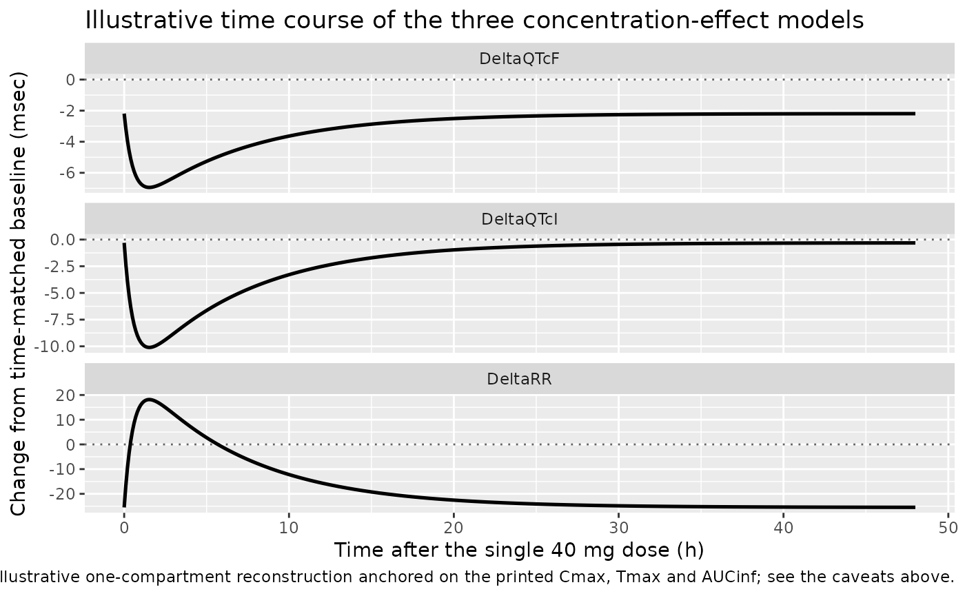
peak_conc_time <- tc_events$time[which.max(tc_events$CP_SAPANISERTIB_NGML)]

stopifnot(
  # The two QTc endpoints reach their most negative value at the same TIME as
  # the concentration peak, and the RR endpoint its most positive: the models
  # are direct-effect, with no hysteresis (the paper checked for hysteresis
  # graphically and found none -- Methods, "Statistical Analyses"). Compared on
  # time rather than row index so the assertion does not depend on the row
  # ordering rxSolve returns.
  with(tc[tc$endpoint == "DeltaQTcI", ], time[which.min(value)]) ==
    peak_conc_time,
  with(tc[tc$endpoint == "DeltaQTcF", ], time[which.min(value)]) ==
    peak_conc_time,
  with(tc[tc$endpoint == "DeltaRR", ], time[which.max(value)]) ==
    peak_conc_time
)
Reconciling the RR model with the reported heart-rate time course
The concentration-DeltaRR fit and the paper’s heart-rate
time course point in apparently opposite directions, and it is worth
being explicit that they do not conflict.
Supplementary Table S1 reports the least-squares-mean change in heart rate rising steadily with time, from -4.4 bpm at 0.5 h to a maximum of +12.4 bpm at 24 h after dosing. But at 24 h the sapanisertib concentration has fallen far below Cmax – roughly 11 ng/mL on the illustrative trajectory above, given the reported 9 h half-life. So the observed net tachycardia occurs when drug concentrations are low, and it is carried in the concentration-effect model by the large negative intercept (-25.5 msec of RR, i.e. a faster heart rate than time-matched baseline at zero concentration), not by the slope. The positive slope acts in the opposite direction, partially offsetting that intercept as concentration rises.
rr_points <- tibble::tibble(
  scenario = c("Zero concentration", "4 mg Cmax", "30 mg Cmax", "40 mg Cmax"),
  conc     = c(0, 36.9, 235.0, 297.0)
) |>
  dplyr::mutate(
    d_rr = predict_endpoint(mod_rr, conc)$d_rr
  )
#> Warning: There was 1 warning in `dplyr::mutate()`.
#> ℹ In argument: `d_rr = predict_endpoint(mod_rr, conc)$d_rr`.
#> Caused by warning:
#> ! multi-subject simulation without without 'omega'

rr_points |>
  dplyr::transmute(
    Scenario                       = scenario,
    `Sapanisertib conc (ng/mL)`    = conc,
    `Model DeltaRR (msec)`         = round(d_rr, 2)
  ) |>
  knitr::kable(
    caption = paste(
      "Model-predicted DeltaRR at zero concentration and at the three",
      "geometric-mean Cmax anchors. The intercept carries an RR shortening",
      "(faster heart rate); the positive slope offsets it as concentration",
      "rises, turning DeltaRR positive above about 174 ng/mL."
    )
)| Scenario | Sapanisertib conc (ng/mL) | Model DeltaRR (msec) |
|---|---|---|
| Zero concentration | 0.0 | -25.50 |
| 4 mg Cmax | 36.9 | -20.08 |
| 30 mg Cmax | 235.0 | 9.04 |
| 40 mg Cmax | 297.0 | 18.15 |
stopifnot(
  # The intercept-only prediction is an RR shortening, and the 40 mg Cmax
  # prediction is an RR lengthening: the sign flip within the studied range is
  # the whole reconciliation, so it is asserted rather than only narrated.
  rr_points$d_rr[rr_points$scenario == "Zero concentration"] < 0,
  rr_points$d_rr[rr_points$scenario == "40 mg Cmax"] > 0
)
Note also that the two analyses use different populations (44 patients for the concentration-effect fits, 32 for the least-squares-mean time course) and different scales (RR interval in msec versus heart rate in bpm, which are reciprocally related), so no quantitative gate between them is appropriate.
Assumptions and deviations
All six parameter values come from regression tables printed inside raster figure panels. Figures 4A and 4C of the article and Figure S2 of the supplement each embed a
Parameter | Estimate | SE | df | t-value | P-value | 95% Bootstrap CItable inside the plot area. These are printed parameter tables and carry full printed-value authority – nothing here was digitised off a curve or fitted – but they are invisible to every text-extraction path. Recovery requiredpdftoppm -r 400 -f 10on the article PDF and unzippingcpdd808-sup-0001-suppmat.docxto renderword/media/image4.png. Reviewers re-checking these values must render the images; grepping the text will find nothing. The verification tables above exist precisely so the transcription can be audited without re-reading the images.Inter-individual variability is not quantified in the source. The Methods state that “Mixed-effects models were subsequently developed to describe the direct effect of sapanisertib on change from time-matched baseline in RR, QTcI, and QTcF”, and the residual degrees of freedom (409, 440, 470 against 44 patients) are consistent with a per-subject random intercept. But no variance estimate, random-effect standard deviation or shrinkage value is reported for any of the three models. Per the maintainers’ standing policy on unreported IIV, the packaged models omit the eta declarations and ship typical-value-only encodings. The only surviving traces of the variance components are Table 4’s threshold-exceedance probability columns and the Figure 4B / 4D 90% prediction intervals; neither inverts to a unique variance, so no value is guessed. Users who need an IIV envelope must impose one externally.
Residual error is not reported numerically.
addSd <- fixed(0)in all three files, per the maintainers’ standing policy, so each model returns its deterministic typical-value prediction. This follows the same encoding asDarpo_2014_racSotalol_QTcI.R/_QTcF.R.Table 4’s exceedance probabilities are deliberately not gated. The paper reports the estimated probability of
DeltaQTc exceeding 30 and 60 msec at each Cmax anchor (at most 0.0139 and 0.0001 respectively). Reproducing those numbers requires the unreported variance components, and back-solving them from the probabilities does not identify a unique variance: the implied total standard deviation is not constant across the three anchors (about 9.7, 14.8 and 18.3 msec at 4, 30 and 40 mg forDeltaQTcI), so the reported probabilities evidently also carry concentration uncertainty, parameter uncertainty, or both. Rather than fit a variance to match a probability column, the gap is recorded here.No structural PK model exists in the source. Sapanisertib PK was characterised by non-compartmental analysis only (geometric mean Cmax 297 ng/mL, AUC-infinity 2480 ng*h/mL, CL/F 16.1 L/h, terminal half-life 9.06 h geometric mean; Supplementary Table S2), and no sapanisertib popPK model exists in the nlmixr2lib registry as of this extraction. All three models therefore consume
CP_SAPANISERTIB_NGML(ng/mL) as a time-varying covariate. The illustrative reconstruction above is a vignette device only, and its 4.6 h implied half-life versus the reported 9.06 h shows a one-compartment form is inadequate for this drug.Three model files, one vignette. The paper fits the three concentration-effect models independently, one per endpoint, with different residual degrees of freedom – they are not sub-models of a joint fit. Per the standing replicate-the-author’s-structure policy that maps to three
.Rfiles and, because they come from one paper, this single vignette.The RR endpoint is named
d_rr, the two QTc endpoints are notd-prefixed. This asymmetry within the file set is deliberate and was a maintainer ruling of 2026-09-02. The register had no RR entry of either form.d_rrwas ratified as a canonical sibling of the existingd_hrchange-from-baseline heart-rate endpoint, on the scale-incomparability grounds that entry already states – an absolute RR interval is roughly 850 msec whereas thisDeltaRR spans -25 to +18 msec – and because the competing bare-name precedent (QTc,QTcF,QTcI) is for absolute interval names. The two QTc siblings keep their bare corrected-interval names in line with the existing registry usage inDarpo_2014_racSotalol_QTcF.R,Mukker_2026_tuvusertib_QTcF.RandZhou_2025_fruquintinib_*; the per-modelunitsfield documents the change-from-baseline semantic in each case.Reported race percentages do not sum to 100. Table 1 lists White 68%, Black 20% and not reported 11%, summing to 99% from independent rounding of 30, 9 and 5 of 44. The
populationmetadata records the printed percentages as given.PKNCA validation is not applicable. PKNCA is the validation surface for drug-concentration endpoints; all three endpoints here are derived electrocardiographic PD quantities in msec, not plasma concentrations, and the paper reports no concentration-time model to run NCA against. The Table 4 zero-parameter gate is the appropriate validation for a linear mixed-effects PD model whose entire content is its coefficient table, and it is supplemented above by the Table-4 inversion cross-check, the panel-table internal-consistency check, and the sign and threshold assertions.