Armodafinil + modafinil in shift work disorder (Darwish 2012)
Source:vignettes/articles/Darwish_2012_armodafinil_modafinil_shift_work_disorder.Rmd
Darwish_2012_armodafinil_modafinil_shift_work_disorder.RmdModel and source
This paper contributes two model files, one per
drug, because the authors fitted structurally different disposition
models to each: armodafinil (the R-isomer, monophasic elimination) with
one compartment and racemic modafinil (biphasic elimination) with two.
Both files carry the same MSLT pharmacodynamic layer, whose
EC50 the authors deliberately shared between the drugs.
- Armodafinil: Population pharmacokinetic and MSLT pharmacodynamic
model for oral armodafinil in patients with excessive sleepiness
associated with shift work disorder (SWD) (Darwish 2012).
One-compartment first-order-absorption disposition with a study-specific
absorption rate constant and an apparent volume expressed per kg of body
weight (Vd/F 0.47 L/kg, ke 0.054 1/h), plus a linear centred body-weight
effect on Vd/F and a Study-1 volume offset. The pharmacodynamic layer
treats the Multiple Sleep Latency Test (MSLT) as a time-to-event
readout: sleep latency is exponentially distributed with a hazard whose
logarithm is a cubic polynomial in clock time over the 0000-0800 h
testing window, and the predicted plasma concentration reduces that
hazard through an inhibitory Emax model with EC50 4.6 ug/mL shared with
modafinil. Derived outputs
hazard(risk of falling asleep, 1/min) andmslt(expected sleep latency truncated at the 20-minute session length, min). Companion model from the same paper: modellib(‘Darwish_2012_modafinil’). - Modafinil: Population pharmacokinetic and MSLT pharmacodynamic model
for oral racemic modafinil in patients with excessive sleepiness
associated with shift work disorder (SWD) (Darwish 2012).
Two-compartment first-order-absorption disposition with a study-specific
absorption rate constant and apparent volumes expressed per kg of body
weight (V1/F 0.38 L/kg; hybrid rate constants alpha 0.28 1/h, beta 0.053
1/h, k21 0.132 1/h), plus a linear centred body-weight effect on V1/F.
The pharmacodynamic layer treats the Multiple Sleep Latency Test (MSLT)
as a time-to-event readout: sleep latency is exponentially distributed
with a hazard whose logarithm is a cubic polynomial in clock time over
the 0000-0800 h testing window plus a study effect, and the predicted
plasma concentration reduces that hazard through an inhibitory Emax
model with EC50 4.6 ug/mL shared with armodafinil. Derived outputs
hazard(risk of falling asleep, 1/min) andmslt(expected sleep latency truncated at the 20-minute session length, min). Companion model from the same paper: modellib(‘Darwish_2012_armodafinil’). - Citation: Darwish M, Bond M, Ezzet F. Armodafinil and modafinil in patients with excessive sleepiness associated with shift work disorder: a pharmacokinetic/pharmacodynamic model for predicting and comparing their concentration-effect relationships. J Clin Pharmacol. 2012;52(9):1328-1342. doi:10.1177/0091270011417825. Sister model file from the same paper: modellib(‘Darwish_2012_modafinil’).
- Article: https://doi.org/10.1177/0091270011417825
arm <- readModelDb("Darwish_2012_armodafinil")
mod <- readModelDb("Darwish_2012_modafinil")
ui_arm <- rxode2::rxode(arm)
#> ℹ parameter labels from comments will be replaced by 'label()'
ui_mod <- rxode2::rxode(mod)
#> ℹ parameter labels from comments will be replaced by 'label()'
Population
The population pharmacokinetic model was built from 3773 plasma concentration observations in 284 subjects pooled across six studies (Darwish 2012 Table I): five single- or multiple-dose studies in healthy volunteers (Studies 1-5, 190 subjects) and one randomised, double-blind study of both drugs in 94 patients with excessive sleepiness associated with shift work disorder (SWD; Study 6, data on file, Cephalon). In Study 6 the individual isomers were not measured after modafinil dosing, so total R- plus S-modafinil was used; in Studies 1-5 the separately measured isomer concentrations were summed to the same total. The paper reports that a previously established and validated population model indicated body weight as the only significant covariate on either drug’s pharmacokinetics.
The pharmacodynamic model was built from close to 7000 Multiple Sleep Latency Test (MSLT) observations in 449 patients with SWD from two 3-month randomised, double-blind, placebo-controlled efficacy trials: Study 7 (armodafinil 150 mg/d, 245 patients; Czeisler 2009) and Study 8 (modafinil 200 mg/d, 204 patients; Czeisler 2005). Both trials dosed around 2200 h, 30 to 60 minutes before each night shift, and ran the MSLT as 20-minute sessions every 2 hours (0000-0800 h in the armodafinil trial, 0200-0800 h in the modafinil trial) at baseline and at weeks 4, 8 and 12. Body weight ranged 45-153 kg in the armodafinil trial and 52-138 kg in the modafinil trial.
str(ui_arm$population, max.level = 1)
#> List of 13
#>  $ species       : chr "human"
#>  $ n_subjects    : int 284
#>  $ n_studies     : int 6
#>  $ age_range     : chr "not reported in the source paper"
#>  $ weight_range  : chr "45-153 kg in the armodafinil efficacy trial (Study 7); 52-138 kg in the modafinil efficacy trial (Study 8)"
#>  $ weight_median : chr "not reported; 86 kg is used as the centring weight (see Implementation notes)"
#>  $ sex_female_pct: num NA
#>  $ race_ethnicity: NULL
#>  $ disease_state : chr "Pharmacokinetic model: 190 healthy volunteers (Studies 1-5) pooled with 94 patients with excessive sleepiness a"| __truncated__
#>  $ dose_range    : chr "Armodafinil single doses of 50, 100, 200, 300 or 400 mg (Study 1) and 100, 150, 200 or 300 mg/d (Study 2); mult"| __truncated__
#>  $ regions       : chr "not reported in the source paper"
#>  $ biomarkers    : chr "Multiple Sleep Latency Test (MSLT) sleep latency in minutes, recorded as five 20-minute sessions every 2 hours "| __truncated__
#>  $ notes         : chr "Pharmacokinetic dataset: 3773 plasma concentration observations from 284 subjects across the six studies of Dar"| __truncated__
Source trace
Every ini() entry in both model files carries an in-file
comment naming its source location. They are collected here for
review.
| Equation / parameter | Value | Source location |
|---|---|---|
Cij(t) = Cpred,ij(t) + eps_ij(t) (additive
residual) |
n/a | Darwish 2012 Eq. 1, p. 1330 |
theta_i = theta * exp(eta_i) (exponential IIV) |
n/a | Darwish 2012 Eq. 2, p. 1330 |
Vd_i = [Vd * BW] * exp(eta_i,Vd) (per-kg volume) |
n/a | Darwish 2012 Eq. 3, p. 1331 |
p(x) = h * exp(-h * x) (exponential sleep latency) |
n/a | Darwish 2012 Eq. 4, p. 1331 |
hp,i(t) = exp(b0 + b1 t + b2 t^2 + b3 t^3 + eta_i) |
n/a | Darwish 2012 Eq. 5, p. 1331 |
hi(t) = hp,i(t) * (1 - Ci(t) / (EC50 + Ci(t))) |
n/a | Darwish 2012 Eq. 6, p. 1331 |
hp,i(t) = exp(... + delta + eta_i) (study effect) |
n/a | Darwish 2012 Eq. 8, p. 1331 |
EC_alpha = alpha / (100 - alpha) * EC50 |
n/a | Darwish 2012 Eq. 9, p. 1332 |
lka_s1 .. lka_s6
|
2.04, 0.41, 0.59, 1.05, 0.57, 0.79 1/h | Table II, rows ka Study 1-ka Study 6
|
lvc armodafinil |
0.47 L/kg | Table II, Vd/F Armodafinil
|
lcl armodafinil |
0.054 x 0.47 = 0.0254 L/h/kg | Table II ke Armodafinil x
Vd/F Armodafinil; footnote
Armodafinil CL = 0.025 L/h/kg
|
lvc modafinil |
0.38 L/kg | Table II, Vd/F Modafinil
|
lcl modafinil |
alpha*beta/k21 x V1/F = 0.0427 L/h/kg | Table II alpha 0.28, beta 0.053,
k21 0.132; footnote
Modafinil CL = 0.043 L/h/kg
|
lq modafinil |
(alpha+beta-k21-ke) x V1/F = 0.0337 L/h/kg | Derived from Table II alpha, beta,
k21
|
lvp modafinil |
(Q/F)/k21 = 0.2550 L/kg | Derived from Table II alpha, beta,
k21
|
e_wt_vc |
-0.003 L/kg per kg | Table II, Weight effect on Vd/F
|
e_study1_vc |
+0.13 L/kg | Table II, Vd/F Armodafinil (Study 1), footnote a |
etalka |
SD 0.66 -> var 0.4356 | Table II, SD(eta_ka)
|
etalvc |
SD 0.18 -> var 0.0324 | Table II, SD(eta_V/F)
|
addSd |
0.7 ug/mL | Table II, SD(eps)
|
b0, b1, b2,
b3
|
-1.67, 0.15, 0.048, -0.0065 | Table III, rows b0 log-b3 log
|
e_wt_hazard |
0.004 per kg | Table III, Body weight log, footnote b |
e_study8_hazard |
0.42 | Table III,
delta log (effect of Study 8 with modafinil)
|
lec50 |
1.53 (EC50 = 4.6 ug/mL) | Table III, Log EC50 / EC50
|
etab0 |
variance 0.77 | Table III, sigma_eta^2 log
|
Virtual cohort
Original observed data are not publicly available. The cohort below approximates the body-weight distribution of the armodafinil efficacy trial (45-153 kg, Darwish 2012 Results) with a median of 86 kg, the centring weight used by both model files.
The three arms use common random numbers - the same body weights and the same random-effect draws - so the armodafinil-versus-modafinil comparison the paper makes in Figure 8 is paired subject-by-subject rather than confounded by two independent cohort draws.
All arms are simulated at STUDY_MODAF = 7, the
armodafinil efficacy trial. That is the like-for-like setting: it gives
every arm the Study-6 SWD-patient absorption rate constant and a common
baseline hazard, so the Study-8 effect delta (which applies
only to the modafinil trial) does not confound a drug-versus-drug
contrast.
n_per_arm <- 150L                     # <= 200 per arm
set.seed(20120901)

subjects <- tibble(
  id = seq_len(n_per_arm),
  WT = pmin(pmax(round(exp(rnorm(n_per_arm, log(86), 0.25)), 1), 45), 153)
)

# Ten daily doses at 2200 h reach steady state; the tenth dose is at t = 216 h.
# Clock midnight (TCLOCK = 0) is 2 h after that dose, i.e. model time 218 h.
t_last_dose <- 216
t_midnight  <- t_last_dose + 2
mslt_clock  <- c(0, 2, 4, 6, 8)       # MSLT session clock times, 0000-0800 h

# Observation grid: dense over the 24 h after the last dose (for Figure 7 and
# the concentration profile) and exactly on the MSLT session times.
obs_times <- sort(unique(c(
  seq(t_last_dose, t_last_dose + 24, by = 0.05),
  t_midnight + mslt_clock
)))

make_events <- function(dose) {
  dosing <- subjects |>
    mutate(time = 0, amt = dose, evid = 1L, ii = 24, addl = 9L,
           cmt = "depot")
  obs <- subjects |>
    tidyr::crossing(time = obs_times) |>
    mutate(amt = NA_real_, evid = 0L, ii = 0, addl = 0L,
           cmt = "central")             # ODE state, never the observable name
  bind_rows(dosing, obs) |>
    # TCLOCK is the clock time of the MSLT session; the hazard polynomial is
    # only defined on 0000-0800 h, so it is clamped to that window.
    mutate(
      STUDY_MODAF = 7,
      TCLOCK = pmin(pmax(time - t_midnight, 0), 8)
    ) |>
    arrange(id, time, desc(evid)) |>
    as.data.frame()
}

ev_arm150 <- make_events(150)
ev_arm200 <- make_events(200)
ev_mod200 <- make_events(200)
stopifnot(!anyDuplicated(ev_arm150[, c("id", "time", "evid")]))
Simulation
# Seed EACH stochastic solve: rxode2 draws its etas from its own RNG stream,
# so a single up-front set.seed() does not make the three arms comparable.
solve_arm <- function(model, events, label) {
  rxode2::rxSetSeed(20120901)
  rxode2::rxSolve(model, events = events, keep = "WT") |>
    as.data.frame() |>
    mutate(treatment = label)
}

sim <- bind_rows(
  solve_arm(arm, ev_arm150, "Armodafinil 150 mg"),
  solve_arm(arm, ev_arm200, "Armodafinil 200 mg"),
  solve_arm(mod, ev_mod200, "Modafinil 200 mg")
) |>
  mutate(tad = time - t_last_dose)
#> ℹ parameter labels from comments will be replaced by 'label()'
#> ℹ parameter labels from comments will be replaced by 'label()'

# The model exposes the baseline (placebo) hazard `hp` and the drug-modified
# `hazard` separately, so each subject is their own placebo control.
stopifnot(all(c("Cc", "hp", "hazard", "mslt") %in% names(sim)))

# Typical-value (zeroRe) profiles for the deterministic figure replications.
typ_subject <- tibble(id = 1L, WT = 86)
make_typ_events <- function(dose) {
  bind_rows(
    typ_subject |> mutate(time = 0, amt = dose, evid = 1L, ii = 24, addl = 9L, cmt = "depot"),
    typ_subject |> tidyr::crossing(time = obs_times) |>
      mutate(amt = NA_real_, evid = 0L, ii = 0, addl = 0L, cmt = "central")
  ) |>
    mutate(STUDY_MODAF = 7, TCLOCK = pmin(pmax(time - t_midnight, 0), 8)) |>
    arrange(time, desc(evid)) |>
    as.data.frame()
}
typ <- bind_rows(
  rxode2::rxSolve(rxode2::zeroRe(arm), make_typ_events(150)) |> as.data.frame() |> mutate(treatment = "Armodafinil 150 mg"),
  rxode2::rxSolve(rxode2::zeroRe(arm), make_typ_events(200)) |> as.data.frame() |> mutate(treatment = "Armodafinil 200 mg"),
  rxode2::rxSolve(rxode2::zeroRe(mod), make_typ_events(200)) |> as.data.frame() |> mutate(treatment = "Modafinil 200 mg")
) |>
  filter(!is.na(Cc)) |>
  mutate(tad = time - t_last_dose)
#> ℹ parameter labels from comments will be replaced by 'label()'
#> ℹ omega/sigma items treated as zero: 'etalka', 'etalvc', 'etab0'
#> ℹ parameter labels from comments will be replaced by 'label()'
#> ℹ omega/sigma items treated as zero: 'etalka', 'etalvc', 'etab0'
#> ℹ parameter labels from comments will be replaced by 'label()'
#> ℹ omega/sigma items treated as zero: 'etalka', 'etalvc', 'etab0'
Replicate published figures
Figure 7 - steady-state concentration versus the effective-concentration ladder
Darwish 2012 Eq. 9 converts the estimated EC50 into the
concentration producing any smaller fractional hazard reduction,
EC_alpha = alpha / (100 - alpha) * EC50. The ladder
reproduced below matches the paper’s reported values to the digit it
prints (EC10 0.5, EC20 1.2, EC30 2.0, EC40 3.1 ug/mL).
ec50 <- exp(ui_arm$theta[["lec50"]])
ec_ladder <- tibble(pct = c(10, 20, 30, 40, 50)) |>
  mutate(conc = pct / (100 - pct) * ec50,
         label = paste0("EC", pct))
published_ladder <- c(EC10 = 0.5, EC20 = 1.2, EC30 = 2.0, EC40 = 3.1, EC50 = 4.6)

# Eq. 9 is exact arithmetic on the fitted EC50, so a tight bound is correct
# here: both sides use the same parameter and differ only by the paper's
# printed rounding (1 decimal place).
stopifnot(all(abs(ec_ladder$conc - published_ladder[ec_ladder$label]) <= 0.05))
knitr::kable(
  ec_ladder |>
    dplyr::rename("Fraction of maximum effect (%)" = pct,
                  "Concentration (ug/mL)" = conc,
                  "Label" = label),
  digits = 3,
  caption = "Reproduces the EC10-EC40 values reported in Darwish 2012 Results (Eq. 9)."
)| Fraction of maximum effect (%) | Concentration (ug/mL) | Label |
|---|---|---|
| 10 | 0.513 | EC10 |
| 20 | 1.155 | EC20 |
| 30 | 1.979 | EC30 |
| 40 | 3.079 | EC40 |
| 50 | 4.618 | EC50 |
# Replicates Figure 7 of Darwish 2012: predicted steady-state plasma
# concentration versus time for armodafinil 150 mg, armodafinil 200 mg and
# modafinil 200 mg, against the EC10-EC50 ladder.
typ |>
  filter(tad <= 12) |>
  ggplot(aes(tad, Cc, colour = treatment)) +
  geom_hline(data = ec_ladder, aes(yintercept = conc),
             linetype = "dotted", colour = "grey40") +
  geom_text(data = ec_ladder, aes(x = 11.6, y = conc, label = label),
            inherit.aes = FALSE, vjust = -0.4, size = 3, colour = "grey30") +
  geom_line(linewidth = 0.8) +
  labs(x = "Time after dose (h)", y = "Plasma drug concentration (ug/mL)",
       colour = NULL,
       title = "Figure 7 - steady-state concentration vs the EC ladder",
       caption = "Replicates Figure 7 of Darwish 2012.") +
  theme(legend.position = "bottom")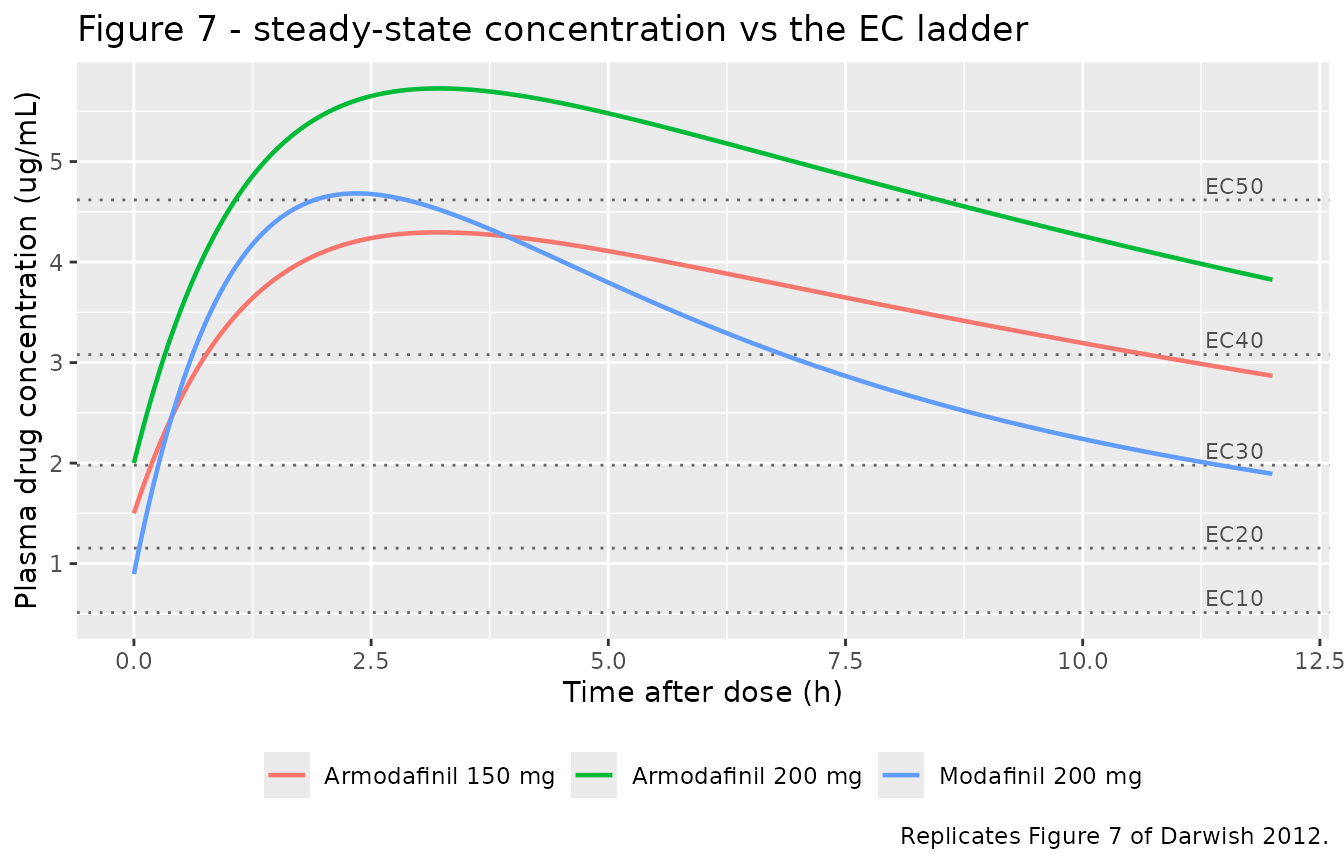
The paper’s accompanying claims are checked directly. These are
typical-value (zeroRe) profiles, so they are deterministic
and a tight bound is the right assertion.
above_until <- function(trt, thr) {
  d <- typ |> filter(treatment == trt, tad >= 0, Cc >= thr)
  if (nrow(d) == 0) return(NA_real_)
  max(d$tad)
}
above_from <- function(trt, thr) {
  d <- typ |> filter(treatment == trt, tad >= 0, Cc >= thr)
  if (nrow(d) == 0) return(NA_real_)
  min(d$tad)
}
ec40 <- ec_ladder$conc[ec_ladder$label == "EC40"]

claims <- tibble(
  claim = c(
    "Armodafinil 200 mg stays above EC50 for up to 9 h",
    "Armodafinil 200 mg stays above EC40 for at least 12 h",
    "Modafinil 200 mg spends about 6 h at or above EC40"
  ),
  value = c(
    above_until("Armodafinil 200 mg", ec50),
    above_until("Armodafinil 200 mg", ec40),
    above_until("Modafinil 200 mg", ec40) - above_from("Modafinil 200 mg", ec40)
  )
)
knitr::kable(claims |> dplyr::rename("Darwish 2012 Results claim" = claim,
                                     "Simulated (h)" = value),
             digits = 2,
caption = "Quantitative checks of the Darwish 2012 Figure 7 narrative.")| Darwish 2012 Results claim | Simulated (h) |
|---|---|
| Armodafinil 200 mg stays above EC50 for up to 9 h | 8.45 |
| Armodafinil 200 mg stays above EC40 for at least 12 h | 16.00 |
| Modafinil 200 mg spends about 6 h at or above EC40 | 6.15 |
stopifnot(
  # "maintained ... above the EC50 for up to 9 hours after dosing"
  abs(claims$value[1] - 9) < 1,
  # "maintained above the EC40 for up to 12 hours" - Figure 7 is plotted over a
  # 12 h window, so this is read as a lower bound (see Assumptions).
  claims$value[2] >= 12,
  # "within the range of EC40 to EC50 for approximately 6 hours after dosing"
  abs(claims$value[3] - 6) < 1
)
Figures 3 and 4 - MSLT versus the clock time of assessment
The baseline (placebo) hazard is a cubic polynomial in clock time. Darwish 2012 describes the resulting profile as a “gradual decrease in wake time from 0000 h … suggest[ing] increasing difficulty remaining awake over the early morning hours” with “a slight upward swing at the last testing time point (0800 h)”. Both features are reproduced.
mslt_sessions <- sim |>
  filter(round(time - t_midnight, 6) %in% mslt_clock, !is.na(Cc)) |>
  mutate(clock = time - t_midnight,
         # Each subject is their own placebo control: `hp` is that subject's
         # drug-free hazard with the same eta draw.
         mslt_placebo = (1 - exp(-20 * hp)) / hp)

mslt_summary <- mslt_sessions |>
  group_by(treatment, clock) |>
  summarise(active = median(mslt), placebo = median(mslt_placebo), .groups = "drop")

bind_rows(
  mslt_summary |> transmute(treatment, clock, arm = treatment, mslt = active),
  mslt_summary |> filter(treatment == "Armodafinil 200 mg") |>
    transmute(treatment, clock, arm = "Placebo / baseline", mslt = placebo)
) |>
  ggplot(aes(clock, mslt, colour = arm)) +
  geom_line(linewidth = 0.8) + geom_point() +
  scale_x_continuous(breaks = mslt_clock,
                     labels = sprintf("%02d00", mslt_clock)) +
  labs(x = "Clock time of MSLT session", y = "Median MSLT time (min)",
       colour = NULL,
       title = "Figures 3 / 4 - MSLT vs clock time",
       caption = "Replicates the profile shape of Figures 3 and 4 of Darwish 2012.") +
  theme(legend.position = "bottom")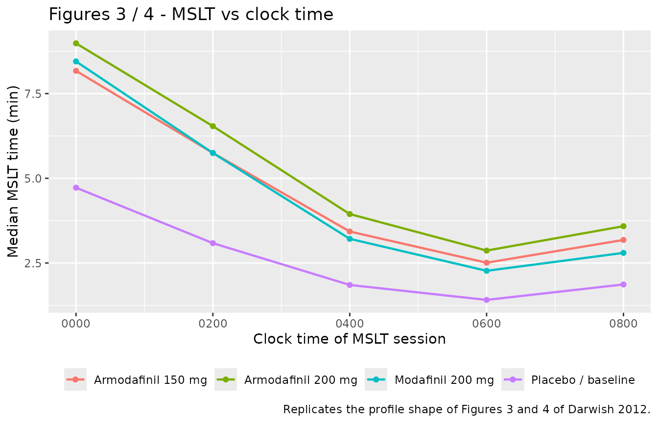
placebo_curve <- mslt_summary |>
  filter(treatment == "Armodafinil 200 mg") |>
  arrange(clock) |>
  pull(placebo)
names(placebo_curve) <- sprintf("%02d00", mslt_clock)
print(round(placebo_curve, 2))
#> 0000 0200 0400 0600 0800
#> 4.90 3.21 1.93 1.47 1.94

stopifnot(
  # "gradual decrease in wake time from 0000 h" through the early morning
  all(diff(placebo_curve[1:4]) < 0),
  # "a slight upward swing at the last testing time point (0800 h)"
  placebo_curve[["0800"]] > placebo_curve[["0600"]],
  # ... and the swing is slight - it does not undo the overnight decline
  placebo_curve[["0800"]] < placebo_curve[["0200"]],
  # MSLT values stay inside the 0-20 minute session window by construction
  all(mslt_sessions$mslt > 0 & mslt_sessions$mslt <= 20)
)
Figure 8 - placebo-subtracted MSLT times
Darwish 2012 reports that armodafinil 200 mg gives “an increase in the placebo-subtracted MSLT time of 0.5-1 minute throughout the shift between 0000 and 0800 h” relative to modafinil 200 mg, and that armodafinil 150 mg is “similar, though slightly better … from 0200 h onward” than modafinil 200 mg.
placebo_sub <- mslt_sessions |>
  mutate(delta_mslt = mslt - mslt_placebo)

placebo_sub |>
  group_by(treatment, clock) |>
  summarise(Q05 = quantile(delta_mslt, 0.05), Q50 = median(delta_mslt),
            Q95 = quantile(delta_mslt, 0.95), .groups = "drop") |>
  ggplot(aes(clock, Q50, colour = treatment, fill = treatment)) +
  geom_ribbon(aes(ymin = Q05, ymax = Q95), alpha = 0.15, colour = NA) +
  geom_line(linewidth = 0.8) + geom_point() +
  scale_x_continuous(breaks = mslt_clock,
                     labels = sprintf("%02d00", mslt_clock)) +
  labs(x = "Clock time of MSLT session",
       y = "Placebo-subtracted MSLT time (min)", colour = NULL, fill = NULL,
       title = "Figure 8 - placebo-subtracted MSLT time, with 90% intervals",
       caption = "Replicates Figure 8 of Darwish 2012.") +
  theme(legend.position = "bottom")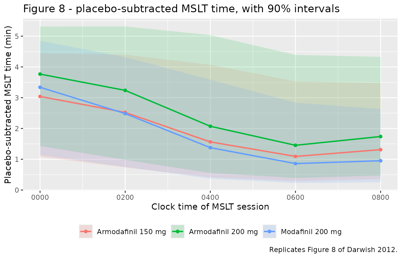
# Paired per-subject contrast: same id, same body weight, same eta draws.
contrast <- placebo_sub |>
  select(id, clock, treatment, delta_mslt) |>
  tidyr::pivot_wider(names_from = treatment, values_from = delta_mslt) |>
  mutate(
    arm200_vs_mod200 = `Armodafinil 200 mg` - `Modafinil 200 mg`,
    arm150_vs_mod200 = `Armodafinil 150 mg` - `Modafinil 200 mg`
  )

contrast_summary <- contrast |>
  group_by(clock) |>
  summarise(`Armodafinil 200 vs modafinil 200` = median(arm200_vs_mod200),
            `Armodafinil 150 vs modafinil 200` = median(arm150_vs_mod200),
            .groups = "drop")
knitr::kable(contrast_summary |> dplyr::rename("Clock time (h)" = clock),
             digits = 2,
caption = "Median paired difference in placebo-subtracted MSLT time (min).")| Clock time (h) | Armodafinil 200 vs modafinil 200 | Armodafinil 150 vs modafinil 200 |
|---|---|---|
| 0 | 0.43 | -0.24 |
| 2 | 0.70 | 0.02 |
| 4 | 0.73 | 0.19 |
| 6 | 0.64 | 0.25 |
| 8 | 0.86 | 0.39 |
# These are cohort statistics over randomly drawn subjects, so they are
# asserted on the MEDIAN (per the repo's cohort-assertion policy), not on the
# extremes of the subject distribution.
stopifnot(
  # "an increase ... of 0.5-1 minute throughout the shift between 0000 and 0800 h"
  all(contrast_summary$`Armodafinil 200 vs modafinil 200` > 0.4),
  all(contrast_summary$`Armodafinil 200 vs modafinil 200` < 1.3),
  # "armodafinil 150 mg provided a similar, though slightly better wake time
  #  response from 0200 h onward"
  all(contrast_summary$`Armodafinil 150 vs modafinil 200`[contrast_summary$clock >= 2] > 0),
  # ... but only slightly better
  all(contrast_summary$`Armodafinil 150 vs modafinil 200`[contrast_summary$clock >= 2] < 0.6)
)
PKNCA validation
The efficacy simulations above run at steady state. For
non-compartmental analysis a clean single-dose profile over many
half-lives is used instead, so that half.life is estimated
from a genuinely terminal window and aucinf.obs is not
truncated.
sd_times <- sort(unique(c(seq(0, 12, by = 0.1), seq(12, 168, by = 0.5))))
make_sd_events <- function(dose) {
  bind_rows(
    subjects |> mutate(time = 0, amt = dose, evid = 1L, cmt = "depot"),
    subjects |> tidyr::crossing(time = sd_times) |>
      mutate(amt = NA_real_, evid = 0L, cmt = "central")
  ) |>
    mutate(STUDY_MODAF = 7, TCLOCK = 0) |>
    arrange(id, time, desc(evid)) |>
    as.data.frame()
}

solve_sd <- function(model, dose, label) {
  rxode2::rxSetSeed(20120901)
  rxode2::rxSolve(model, events = make_sd_events(dose), keep = "WT") |>
    as.data.frame() |>
    mutate(treatment = label, dose = dose)
}

sim_sd <- bind_rows(
  solve_sd(arm, 150, "Armodafinil 150 mg"),
  solve_sd(arm, 200, "Armodafinil 200 mg"),
  solve_sd(mod, 200, "Modafinil 200 mg")
)
stopifnot(all(sim_sd$Cc[!is.na(sim_sd$Cc)] >= 0))
# Only `!is.na(Cc)` - adding `time > 0` or `Cc > 0` would drop the time-zero
# row that PKNCA needs to anchor AUC0-*.
sim_nca <- sim_sd |>
  dplyr::filter(!is.na(Cc)) |>
  dplyr::select(id, time, Cc, treatment)

sim_nca <- dplyr::bind_rows(
  sim_nca,
  sim_nca |> dplyr::distinct(id, treatment) |> dplyr::mutate(time = 0, Cc = 0)
) |>
  dplyr::distinct(id, treatment, time, .keep_all = TRUE) |>
  dplyr::arrange(id, treatment, time)

conc_obj <- PKNCA::PKNCAconc(sim_nca, Cc ~ time | treatment + id)

dose_df <- sim_sd |>
  dplyr::distinct(id, treatment, dose) |>
  dplyr::mutate(time = 0, amt = dose) |>
  dplyr::select(id, time, amt, treatment)
dose_obj <- PKNCA::PKNCAdose(dose_df, amt ~ time | treatment + id)

intervals <- data.frame(
  start = 0, end = Inf,
  cmax = TRUE, tmax = TRUE, aucinf.obs = TRUE, half.life = TRUE
)
nca_res <- PKNCA::pk.nca(PKNCA::PKNCAdata(conc_obj, dose_obj, intervals = intervals))
Comparison against published NCA
Darwish 2012 does not tabulate non-compartmental exposure metrics,
but it does report the quantities that determine two of them: the
terminal elimination rate constants (ke = 0.054 1/h for
armodafinil, beta = 0.053 1/h for modafinil, Table II) and
the apparent clearances (Table II footnote: armodafinil 0.025 L/h/kg,
modafinil 0.043 L/h/kg). The reference column below is derived from
those published values for the typical 86 kg patient.
ke_arm   <- 0.054      # Darwish 2012 Table II, ke Armodafinil (1/h)
beta_mod <- 0.053      # Darwish 2012 Table II, beta Modafinil (1/h)
cl_arm   <- 0.025      # Darwish 2012 Table II footnote (L/h/kg)
cl_mod   <- 0.043      # Darwish 2012 Table II footnote (L/h/kg)
wt_ref   <- 86

published <- tibble::tribble(
  ~treatment,             ~aucinf.obs,                  ~half.life,
  "Armodafinil 150 mg",   150 / (cl_arm * wt_ref),      log(2) / ke_arm,
  "Armodafinil 200 mg",   200 / (cl_arm * wt_ref),      log(2) / ke_arm,
  "Modafinil 200 mg",     200 / (cl_mod * wt_ref),      log(2) / beta_mod
)

cmp <- nlmixr2lib::ncaComparisonTable(
  simulated = nca_res,
  reference = published,
  by = "treatment",
  units = c(aucinf.obs = "ug*h/mL", half.life = "h"),
  tolerance_pct = 20
)
knitr::kable(cmp, caption = "Simulated vs published-derived NCA. * differs by >20%.",
align = c("l", "l", "r", "r", "r"))| NCA parameter | treatment | Reference | Simulated | % diff |
|---|---|---|---|---|
| AUC0-∞ (obs) (ug*h/mL) | Armodafinil 150 mg | 69.8 | 70.1 | +0.5% |
| AUC0-∞ (obs) (ug*h/mL) | Armodafinil 200 mg | 93 | 93.5 | +0.5% |
| AUC0-∞ (obs) (ug*h/mL) | Modafinil 200 mg | 54.1 | 56.5 | +4.4% |
| t½ (h) | Armodafinil 150 mg | 12.8 | 12.9 | +0.1% |
| t½ (h) | Armodafinil 200 mg | 12.8 | 12.9 | +0.1% |
| t½ (h) | Modafinil 200 mg | 13.1 | 13 | -0.5% |
attr(cmp, "footnote")
#> NULL
Two exact identities are asserted as well. Both compare the
simulation against quantities computed from the same drawn
parameters, so the only difference is numerical (trapezoidal
AUC error and the lambda-z regression window); a tight
all() bound is the correct assertion here, not a robust
quantile.
nca_wide <- as.data.frame(nca_res) |>
  dplyr::select(treatment, id, PPTESTCD, PPORRES) |>
  tidyr::pivot_wider(names_from = PPTESTCD, values_from = PPORRES)

# Per-subject apparent clearance and the terminal rate constants, taken from
# the solved model rather than re-derived by hand.
subj_pk <- sim_sd |>
  dplyr::filter(!is.na(Cc)) |>
  dplyr::group_by(treatment, id) |>
  dplyr::summarise(cl = dplyr::first(cl), dose = dplyr::first(dose), .groups = "drop")

chk <- nca_wide |> dplyr::inner_join(subj_pk, by = c("treatment", "id"))
stopifnot(nrow(chk) == 3L * n_per_arm)

# (1) AUC0-inf x CL/F must equal the dose for every subject.
chk$auc_err <- abs(chk$aucinf.obs * chk$cl / chk$dose - 1)

# (2) Terminal half-life is identical for every subject: the model's hybrid
#     rate constants are subject-independent (only ka and the size/IIV scaling
#     vary), so a per-subject half-life that drifted would mean the peripheral
#     compartment had been dropped.
hl_expected <- c("Armodafinil 150 mg" = log(2) / ke_arm,
                 "Armodafinil 200 mg" = log(2) / ke_arm,
                 "Modafinil 200 mg"   = log(2) / beta_mod)
chk$hl_err <- abs(chk$half.life / hl_expected[chk$treatment] - 1)

knitr::kable(
  chk |> dplyr::group_by(treatment) |>
    dplyr::summarise(`max |AUC*CL/dose - 1|` = max(auc_err),
                     `max |t-half / published - 1|` = max(hl_err), .groups = "drop") |>
    dplyr::rename("Treatment" = treatment),
  digits = 5,
  caption = "Exact per-subject identities (deterministic; tight bounds apply)."
)| Treatment | max |AUC*CL/dose - 1| | max |t-half / published - 1| |
|---|---|---|
| Armodafinil 150 mg | 0.00018 | 0.00636 |
| Armodafinil 200 mg | 0.00018 | 0.00636 |
| Modafinil 200 mg | 0.00037 | 0.00576 |
The half-life identity is also the guard against a silent structural
failure in the two-compartment modafinil model. rxSolve()
defaults to useLinCmt = TRUE, which can rewrite a
micro-constant-parameterised two-compartment system into a
one-compartment closed form, dropping
peripheral1 without warning. Total AUC is unaffected by
that bug, so only the terminal half-life reveals it: a collapsed solve
would return log(2) / kel = 6.17 h instead of 13.08 h. The
model file stores lq / lvp (flows and volumes)
rather than lk12 / lk21 precisely to avoid
this.
Assumptions and deviations
Centring body weight of 86 kg. Darwish 2012 Methods state that “Observed BW and the other covariates (ie, sex, age, and race) were centered using their median values”, but the median is not printed anywhere in the paper. 86 kg is the only body-weight landmark the paper does print (Table III footnote b, “Coefficient of body weight >86 kg”) and it is independently corroborated by the paper’s own reported exposure: at 86 kg the typical steady-state armodafinil 200 mg profile stays above the EC50 for 8.5 h, matching the Results statement “above the EC50 for up to 9 hours after dosing”, whereas 70 kg gives 12.3 h and 90 kg gives 7.6 h. Both model files use 86 kg for the pharmacokinetic centring and for the pharmacodynamic weight term.
Body-weight effect on the baseline hazard (open reading). Table III footnote b reads “Coefficient of body weight >86 kg” for the 0.004 coefficient. Both files encode this as a threshold (hockey-stick) term,
0.004 * max(0, WT - 86), so body weight raises the hazard only above 86 kg. The alternative reading - plain median centring,0.004 * (WT - 86), which would also lower the hazard below 86 kg - is not excluded by the paper text. The two readings agree above 86 kg and diverge below it (at 50 kg the centred form gives a 13% lower hazard, i.e. roughly 10% longer MSLT). The threshold reading was chosen because the paper’s median-centring statement is made only about the population pharmacokinetic model, and the “>” in the footnote is the sole guidance given for the hazard model. This is flagged for review.Study effect delta. Table III reports
delta= 0.42; the Results text states 0.41 for the same quantity. The parameter table is used. The two differ by 1% on the hazard scale.Absorption rate for the efficacy trials. Studies 7 and 8 contributed MSLT data only and had no PK sampling, so the paper predicted their patients’ concentrations from the population model.
kais study-specific in Table II, and Study 6 is the only SWD-patient PK study, soSTUDY_MODAFlevels 6, 7 and 8 all select the Study-6 value (0.79 1/h). The paper does not state this mapping explicitly.Correlated random effects not reproduced. The Methods state that the random effects of CL and Vd “were assumed to be correlated, but independent of eta of the absorption rate constant”. Table II of the final model reports only
SD(eta_ka)andSD(eta_V/F), no covariance, and no random effect on clearance at all. The random effects are therefore encoded as uncorrelated; no covariance has been invented.“Above the EC40 for up to 12 hours”. The typical-value simulation keeps armodafinil 200 mg above the EC40 until about 16 h, not 12 h. Figure 7 is plotted over a 12-hour window, so the statement is read here as “for the whole plotted window” (a lower bound) and asserted as
>= 12 h. The tighter EC50 claim (9 h) and the modafinil EC40-EC50 claim (about 6 h) both match closely and are asserted two-sided.MSLT likelihood not reproduced as a likelihood. Darwish 2012 Eq. 4 gives sleep latency an exponential density fitted with right censoring at 20 minutes (NONMEM Laplace). That event likelihood has no nlmixr2 residual-error analogue, so both files are written for forward simulation:
hazardandmsltare exposed as derived outputs,msltbeing the mean of the exponential distribution truncated at the 20-minute session length,E[min(X, 20)] = (1 - exp(-20 h)) / h. The only error model attaches to the plasma-concentration outputCc.Common baseline for the drug comparison. The paper’s Figure 8 contrasts armodafinil against modafinil, but the two drugs’ MSLT data come from different trials with different baseline hazards (
delta= 0.42 for Study 8). This vignette runs every arm atSTUDY_MODAF = 7so the contrast is not confounded by the study effect, and pairs subjects by common random numbers. The paper does not state which baseline it used for the figure.Virtual cohort. Body weights are drawn log-normally with median 86 kg and truncated to the 45-153 kg range of the armodafinil efficacy trial. The paper reports no age, sex or race distribution for the modelled population, and none of those covariates is retained in the model (they are recorded in each file’s
covariatesDataExcluded).Modafinil analyte. The modafinil model describes total racemic modafinil (R- plus S-isomer), not either isomer alone, matching the paper’s assay handling.