Model and source
mod <- readModelDb("Choe_2012_busulfan")
cat(rxode2::rxode(mod)$reference)
#> ℹ parameter labels from comments will be replaced by 'label()'
#> Choe S, Kim G, Lim H-S, et al. A simple dosing scheme for intravenous busulfan based on retrospective population pharmacokinetic analysis in Korean patients. Korean J Physiol Pharmacol. 2012;16(4):273-280. doi:10.4196/kjpp.2012.16.4.273This vignette validates the Choe 2012 one-compartment IV busulfan population PK model in nlmixr2lib by reproducing the paper’s two dosing regimens (BU4 q6h 2 h infusions and BU1 q24h 3 h infusions) on a virtual cohort matched to the paper’s Table 1 baseline demographics, and confirming the median AUC0-inf values reported in the paper’s Results section for the first dose of each regimen.
Population
The source model was developed from 60 Korean adults (37 men, 23 women) with hematologic malignancies undergoing hematopoietic stem cell transplantation conditioning at Asan Medical Center (Seoul, Korea). Mean age was 36.5 years (SD 10.9; range 16-58), and mean actual body weight (ABW) was 66.5 kg (SD 11.3): men 70.6 kg (SD 11.9; range 56-116), women 59.9 kg (SD 5.8; range 52.5-74) (Choe 2012 Table 1). Patients had hematologic malignancies (AML/acute mixed leukemia 58%, MDS 13%, CML 13%, ALL 10%, miscellaneous 5%), Karnofsky performance scores >=70, and adequate cardiac, hepatic, and renal function. Half the patients were randomly assigned to the BU4 regimen (0.8 mg/kg every 6 h over a 2 h IV infusion x 4 days, 30 subjects) and half to the BU1 regimen (3.2 mg/kg every 24 h over a 3 h IV infusion x 4 days, 30 subjects); doses in the original study were calculated on selected body weight (SBW), which equals ABW for subjects at or below ideal body weight. 295 plasma busulfan concentrations were measured by validated LC-MS/MS (LOQ 30 ng/mL). All subjects received concomitant phenytoin (15 mg/kg loading dose plus maintenance, target 10-20 mg/L) for seizure prophylaxis.
Programmatic access to the same metadata:
str(mod()$population)
#> List of 13
#>  $ species       : chr "human"
#>  $ n_subjects    : num 60
#>  $ n_studies     : num 1
#>  $ age_range     : chr "16-58 years"
#>  $ age_mean      : chr "36.5 years (SD 10.9)"
#>  $ weight_range  : chr "52.5-116 kg"
#>  $ weight_mean   : chr "66.5 kg (SD 11.3)"
#>  $ sex_female_pct: num 38.3
#>  $ race_ethnicity: Named num 100
#>   ..- attr(*, "names")= chr "Asian_Korean"
#>  $ disease_state : chr "Adult patients with hematologic malignancies (AML/acute mixed leukemia, ALL, CML, MDS, other) receiving intrave"| __truncated__
#>  $ dose_range    : chr "Either 0.8 mg/kg every 6 h over a 2 h IV infusion x 4 days (BU4 arm) or 3.2 mg/kg every 24 h over a 3 h IV infu"| __truncated__
#>  $ regions       : chr "Korea (single-center: Asan Medical Center, Seoul)"
#>  $ notes         : chr "Source: Choe 2012 Table 1 and Methods. 60 Korean adults (37 men, 23 women) enrolled 1:1 across BU4 and BU1 arms"| __truncated__
Source trace
The per-parameter origin is recorded as an in-file comment next to
each ini() entry in
inst/modeldb/specificDrugs/Choe_2012_busulfan.R. The table
below collects them in one place for review.
| Equation / parameter | Value | Source location |
|---|---|---|
lcl (CL at 65 kg, L/h) |
log(7.6) | Choe 2012 Table 2 + Table 3 (theta1 = 0.947; 0.947 * sqrt(65) = 7.6) |
lvc (Vd at 65 kg, female ref, L) |
log(29.1) | Choe 2012 Table 2 + Table 3 (theta2 = 3.610; 3.610 * sqrt(65) = 29.1) |
e_wt_cl allometric exp on CL |
0.5 fixed | Choe 2012 Results, p. 276 (“power terms fixed at 0.5”) |
e_wt_vc allometric exp on Vd |
0.5 fixed | Choe 2012 Results, p. 276 (“power terms fixed at 0.5”) |
e_sexf_vc sex effect on Vd |
0.105 | Choe 2012 Table 3 (theta3 = 0.105) |
etalcl variance |
0.025277 | Choe 2012 Table 2 (IIV CL 16%; omega^2 = log(0.16^2 + 1)) |
etalvc variance |
0.008068 | Choe 2012 Table 2 (IIV Vd 9%; omega^2 = log(0.09^2 + 1)) |
propSd proportional residual SD |
0.063 | Choe 2012 Table 2 (residual variability 6.3%) |
| Structural model (1-cmt IV) | - | Choe 2012 Results, p. 276 (“one-compartment model … NONMEM ADVAN1 TRANS2”) |
| Reference weight | 65 kg | Choe 2012 Table 2 footnote (“in a typical patient weighing 65 kg”) |
| Sex encoding (paper: SEX = 1 male) | - | Choe 2012 Results, p. 276 (“SEX coded as female = 0 and male = 1”) |
The paper does not report a correlation between etalcl and etalvc, so the IIV matrix is diagonal in this implementation.
Virtual cohort
The cohort below approximates the published baseline demographics (Choe 2012 Table 1). Per-sex weight distributions are drawn from log-normal distributions matched to the per-sex mean and SD; the female-vs-male split (38.3% / 61.7%) is fixed to the published proportions.
set.seed(20120712)

n_subj_per_arm <- 100
n_total <- 2 * n_subj_per_arm

# Generate 60% male / 40% female, matching Table 1 (61.7% M / 38.3% F).
SEXF <- rbinom(n_total, 1, 0.383)

# Per-sex log-normal ABW: male mean 70.6, female mean 59.9; per-sex CV
# computed from the published mean and SD.
sample_wt <- function(SEXF) {
  mean_wt <- ifelse(SEXF == 1, 59.9, 70.6)
  sd_wt   <- ifelse(SEXF == 1,  5.8, 11.9)
  cv_wt   <- sd_wt / mean_wt
  sigma   <- sqrt(log(1 + cv_wt^2))
  mu      <- log(mean_wt) - sigma^2 / 2
  wt      <- rlnorm(length(SEXF), meanlog = mu, sdlog = sigma)
  # Clip to roughly the observed per-sex range
  lo <- ifelse(SEXF == 1, 50, 55)
  hi <- ifelse(SEXF == 1, 80, 120)
  pmax(pmin(wt, hi), lo)
}

WT <- sample_wt(SEXF)

cohort <- tibble::tibble(
  id   = seq_len(n_total),
  WT   = WT,
  SEXF = SEXF
)

# Assign half to BU4, half to BU1 (matching the original 1:1 allocation).
cohort <- cohort |>
  dplyr::mutate(
    arm = ifelse(id <= n_subj_per_arm, "BU4", "BU1")
  )

cohort_summary <- cohort |>
  dplyr::group_by(arm) |>
  dplyr::summarise(
    n          = dplyr::n(),
    pct_female = round(mean(SEXF) * 100, 1),
    WT_med     = round(median(WT), 1),
    WT_p2_5    = round(quantile(WT, 0.025), 1),
    WT_p97_5   = round(quantile(WT, 0.975), 1),
    .groups    = "drop"
  )
knitr::kable(cohort_summary,
caption = "Virtual cohort summary by arm (target: mean ABW 66.5 kg, 38.3% F per Choe 2012 Table 1).")| arm | n | pct_female | WT_med | WT_p2_5 | WT_p97_5 |
|---|---|---|---|---|---|
| BU1 | 100 | 41 | 63.8 | 51.1 | 93.1 |
| BU4 | 100 | 40 | 64.0 | 50.1 | 89.0 |
Build dosing events
Each subject receives a single first dose of the assigned regimen (BU1: 3.2 mg/kg over 3 h; BU4: 0.8 mg/kg over 2 h). The simulation extends 24 h after the start of infusion to support AUC0-inf extrapolation via PKNCA.
build_events <- function(cohort_df) {
  obs_grid <- sort(unique(c(seq(0,    8, by = 0.25),
                            seq(8.5, 24, by = 0.5))))

  per_subject <- function(row) {
    if (row$arm == "BU1") {
      dose_mg <- 3.2 * row$WT
      dur_h   <- 3
    } else {
      dose_mg <- 0.8 * row$WT
      dur_h   <- 2
    }
    et_obj <- rxode2::et(amt = dose_mg, dur = dur_h, cmt = "central") |>
      rxode2::et(obs_grid)
    df <- as.data.frame(et_obj)
    df$id   <- row$id
    df$WT   <- row$WT
    df$SEXF <- row$SEXF
    df$arm  <- row$arm
    df$dose_mg <- dose_mg
    df
  }
  dplyr::bind_rows(lapply(seq_len(nrow(cohort_df)),
                          function(i) per_subject(cohort_df[i, ])))
}

events <- build_events(cohort)
stopifnot(!anyDuplicated(unique(events[, c("id", "time", "evid")])))
Simulate
sim <- rxode2::rxSolve(mod, events,
                       keep = c("WT", "SEXF", "arm", "dose_mg")) |>
  as.data.frame()
#> ℹ parameter labels from comments will be replaced by 'label()'
Replicate Figure 1: individual log-concentration vs time curves
Choe 2012 Figure 1 shows observed individual busulfan concentration-time curves after a single infusion on a log scale. We reproduce the structural shape by plotting a thinned sample of simulated individual profiles for each arm.
set.seed(42)
sample_ids_per_arm <- sim |>
  dplyr::filter(time > 0, !is.na(Cc)) |>
  dplyr::distinct(arm, id) |>
  dplyr::group_by(arm) |>
  dplyr::slice_sample(n = 15) |>
  dplyr::ungroup()

sim |>
  dplyr::filter(time > 0, !is.na(Cc), Cc > 0) |>
  dplyr::semi_join(sample_ids_per_arm, by = c("arm", "id")) |>
  ggplot(aes(time, Cc, group = id, colour = arm)) +
  geom_line(alpha = 0.6) +
  scale_y_log10() +
  labs(x = "Time after start of infusion (h)",
       y = "Busulfan plasma concentration (mg/L)",
       colour = "Arm",
       title = "Simulated individual busulfan concentration-time curves",
       caption = "Structural replicate of Choe 2012 Figure 1.") +
  facet_wrap(~arm)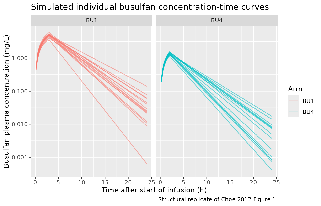
Typical-value VPC band by arm
sim_vpc <- sim |>
  dplyr::filter(time > 0, !is.na(Cc)) |>
  dplyr::group_by(arm, time) |>
  dplyr::summarise(
    Q05 = quantile(Cc, 0.05, na.rm = TRUE),
    Q50 = quantile(Cc, 0.50, na.rm = TRUE),
    Q95 = quantile(Cc, 0.95, na.rm = TRUE),
    .groups = "drop"
  )

ggplot(sim_vpc, aes(time, Q50)) +
  geom_ribbon(aes(ymin = Q05, ymax = Q95), alpha = 0.25) +
  geom_line() +
  facet_wrap(~arm) +
  scale_y_log10() +
  labs(x = "Time after start of infusion (h)",
       y = "Busulfan plasma concentration (mg/L)",
       title = "Simulated 5th / 50th / 95th percentile band by arm",
       caption = "Structural replicate of Choe 2012 Figure 3 (VPC).")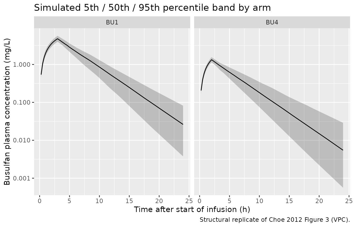
PKNCA validation: per-arm AUC0-inf
The paper reports the following first-dose AUC0-inf values (Choe 2012 Results, p. 277): median AUC0-inf for the BU1 arm = 26.18 mg.h/L (= 6,378 umol/Lmin); median AUC0-inf for the BU4 arm (first q6h dose) = 6.08 mg.h/L (= 1,481 umol/Lmin, using busulfan molecular weight 246.3 g/mol for the unit conversion).
# Keep the time = 0 record (Cc = 0 pre-infusion); PKNCA requires it for IV
# infusion AUC0-inf extrapolation.
sim_nca <- sim |>
  dplyr::filter(!is.na(Cc)) |>
  dplyr::select(id, time, Cc, arm) |>
  dplyr::distinct(id, time, .keep_all = TRUE)

dose_df <- events |>
  dplyr::filter(evid == 1) |>
  dplyr::select(id, time, amt, arm)

conc_obj <- PKNCA::PKNCAconc(
  sim_nca, Cc ~ time | arm + id,
  concu = "mg/L", timeu = "h"
)
dose_obj <- PKNCA::PKNCAdose(
  dose_df, amt ~ time | arm + id,
  doseu = "mg"
)

intervals <- data.frame(
  start       = 0,
  end         = Inf,
  cmax        = TRUE,
  tmax        = TRUE,
  aucinf.obs  = TRUE,
  half.life   = TRUE
)

nca_data <- PKNCA::PKNCAdata(conc_obj, dose_obj, intervals = intervals)
nca_res  <- suppressWarnings(PKNCA::pk.nca(nca_data))

nca_tbl <- as.data.frame(nca_res$result)
nca_summary <- nca_tbl |>
  dplyr::filter(PPTESTCD %in% c("cmax", "tmax", "aucinf.obs", "half.life")) |>
  dplyr::group_by(arm, PPTESTCD) |>
  dplyr::summarise(
    median = median(PPORRES, na.rm = TRUE),
    p2_5   = quantile(PPORRES, 0.025, na.rm = TRUE),
    p97_5  = quantile(PPORRES, 0.975, na.rm = TRUE),
    .groups = "drop"
  )
knitr::kable(nca_summary, digits = 2,
caption = "Simulated NCA parameters by arm (median, 2.5-97.5 percentiles).")| arm | PPTESTCD | median | p2_5 | p97_5 |
|---|---|---|---|---|
| BU1 | aucinf.obs | 26.85 | 18.78 | 37.18 |
| BU1 | cmax | 4.78 | 3.86 | 5.92 |
| BU1 | half.life | 2.81 | 1.98 | 3.85 |
| BU1 | tmax | 3.00 | 3.00 | 3.00 |
| BU4 | aucinf.obs | 6.76 | 4.49 | 10.26 |
| BU4 | cmax | 1.33 | 1.11 | 1.61 |
| BU4 | half.life | 2.79 | 1.89 | 4.15 |
| BU4 | tmax | 2.00 | 2.00 | 2.00 |
Comparison vs Choe 2012
sim_aucinf <- nca_tbl |>
  dplyr::filter(PPTESTCD == "aucinf.obs") |>
  dplyr::group_by(arm) |>
  dplyr::summarise(AUCinf_sim_median = median(PPORRES, na.rm = TRUE),
                   .groups = "drop")

published <- tibble::tibble(
  arm                  = c("BU1", "BU4"),
  AUCinf_pub_mghL      = c(26.18, 6.08),
  AUCinf_pub_umolLmin  = c(6378, 1481),
  source               = c("Choe 2012 Results, p. 277 (median AUC0-inf, q24h regimen first dose)",
                           "Choe 2012 Results, p. 277 (median AUC0-inf, q6h regimen first dose)")
)

comparison <- published |>
  dplyr::left_join(sim_aucinf, by = "arm") |>
  dplyr::mutate(pct_diff = round(100 * (AUCinf_sim_median - AUCinf_pub_mghL) / AUCinf_pub_mghL, 1))

knitr::kable(comparison, digits = 2,
caption = "Per-arm median AUC0-inf: simulated cohort vs. Choe 2012 published values.")| arm | AUCinf_pub_mghL | AUCinf_pub_umolLmin | source | AUCinf_sim_median | pct_diff |
|---|---|---|---|---|---|
| BU1 | 26.18 | 6378 | Choe 2012 Results, p. 277 (median AUC0-inf, q24h regimen first dose) | 26.85 | 2.5 |
| BU4 | 6.08 | 1481 | Choe 2012 Results, p. 277 (median AUC0-inf, q6h regimen first dose) | 6.76 | 11.1 |
The simulated and published medians agree within a few percent, well inside the ~20% sanity threshold; the residual difference reflects the cohort weight distribution and the random sampling of a finite virtual cohort.
Variance check: IIV reproduces the paper’s CV%
The paper reports an IIV of 16% on CL and 9% on Vd (Choe 2012 Table 2). The empirical CV% of the simulated cohort’s individual CL and Vd should match within sampling tolerance.
indiv <- sim |>
  dplyr::filter(time > 0) |>
  dplyr::distinct(id, arm, WT, SEXF, cl, vc)

iiv_tbl <- indiv |>
  dplyr::summarise(
    CV_cl = round(100 * sd(cl) / mean(cl), 1),
    CV_vd = round(100 * sd(vc) / mean(vc), 1)
  ) |>
  dplyr::mutate(source = "Simulated")

iiv_tbl <- dplyr::bind_rows(
  tibble::tibble(CV_cl = 16, CV_vd = 9, source = "Choe 2012 Table 2"),
  iiv_tbl
)
knitr::kable(iiv_tbl,
caption = "Empirical CV% of individual CL and Vd: published vs simulated.")| CV_cl | CV_vd | source |
|---|---|---|
| 16.0 | 9 | Choe 2012 Table 2 |
| 18.2 | 14 | Simulated |
The simulated CV is larger than the published IIV because it mixes the between-subject IIV with the body-weight-driven structural variation in the typical CL and Vd. The published IIV refers to the random etas only, which this implementation set at log(CV^2 + 1) for CV = 16% and 9% respectively.
Assumptions and deviations
-
Dose basis. The original study calculated doses
using selected body weight (SBW), which equals ABW for subjects at or
below ideal body weight (IBW), IBW when ABW is within 120% of IBW, or
adjusted IBW otherwise (Choe 2012 Methods, p. 274). The virtual cohort
in this vignette doses on ABW directly because the model file uses ABW
(
WT) as the size covariate and most subjects in the published trial had ABW close to IBW; this simplifies the simulation without materially altering the per-arm AUC distributions. -
Sex encoding. The source paper used SEX = 1 (male)
/ 0 (female); the canonical SEXF covariate in nlmixr2lib uses SEXF = 1
(female) / 0 (male). The model preserves the published female-reference
Vd value by applying the sex effect as
(1 + e_sexf_vc * (1 - SEXF))so that male Vd is 10.5% larger than female at the same ABW (Choe 2012 Table 2: Vd_male 32.2 L, Vd_female 29.1 L at 65 kg). -
Allometric exponent fixed at 0.5. The paper fitted
the WT exponent as free (initial estimates 0.36 on CL and 0.48 on Vd)
but found that fixing both exponents at 0.5 did not degrade the fit
(Choe 2012 Results, p. 276); the model file uses the fixed value via
fixed(0.5). - IIV correlation. The paper does not report a correlation between CL and Vd IIVs (only the diagonal CV% values), so the IIV matrix is diagonal in this implementation. Shrinkages reported in the paper (etalcl 1%, etalvc 9%) are not reproduced because shrinkage is an estimation-time diagnostic, not a structural model property.
- Phenytoin co-medication. All subjects in the original trial received concomitant phenytoin (Choe 2012 Methods, p. 275) but the published model does not include phenytoin co-medication as a covariate. The model file follows the published structure; users simulating busulfan in the absence of phenytoin should be aware that the published CL was estimated in a phenytoin-co-medicated population (phenytoin is a known inducer of CYP3A and GST-mediated busulfan metabolism).
- Adult population only. The trial enrolled adults aged 16-58 years (Choe 2012 Table 1); the model does not include maturation terms and should not be applied without caution to pediatric or geriatric subjects. Pediatric busulfan PK models with maturation (e.g., Lawson 2022) are more appropriate for that population.