FLT3L-Fc minimal PBPK/PD with expansion-enhanced TMDD (Hosseini 2024)
Source:vignettes/articles/Hosseini_2024_flt3lfc.Rmd
Hosseini_2024_flt3lfc.RmdModel and source
- Article: https://doi.org/10.3390/pharmaceutics16050660 (Pharmaceutics 2024;16(5):660, PMCID PMC11125320)
- Supplement: https://www.mdpi.com/article/10.3390/pharmaceutics16050660/s1 — Table S1 (studies), Table S2 (all model parameters), “Supplemental ODEs and Repeated Assignments” (the SimBiology ODE export), and the SimBiology/gQSPSim project itself.
Hosseini and colleagues built a minimal physiologically based PK/PD (minPBPK/PD) model for FLT3L-Fc (RO7497987), a half-life-extended, effectorless Fc fusion of human FLT3 ligand, to select the first-in-human (FIH) dose. The distinguishing mechanism is expansion-enhanced target-mediated drug disposition: FLT3L-Fc binds one or two monomeric FLT3 receptors in plasma, and the double-bound (homodimer) complex drives proliferation of FLT3-bearing progenitors, expanding the total receptor pool and so amplifying its own TMDD.
The paper contributes two models to nlmixr2lib, matching
the way the authors built them:
cyno  <- readModelDb("Hosseini_2024_flt3lfc_cyno")
human <- readModelDb("Hosseini_2024_flt3lfc_human")

modCyno  <- rxode2::rxode2(cyno)
modHuman <- rxode2::rxode2(human)-
Hosseini_2024_flt3lfc_cyno— the minPBPK/TMDD PK model calibrated to cynomolgus monkey data (Table S2, Cyno Value column). Seven states. -
Hosseini_2024_flt3lfc_human— the human translation (Table S2, Human Value column). It carries the same minPBPK/TMDD block plus the empirical CDX-301 PK sub-model and the shared dendritic-cell expansion PD block, exactly as the single published SimBiology model does. Sixteen states.
The two are separate files because they are not merely two parameter
columns of one structure: the cynomolgus model has no PD arm at all
(every CDX-301 and dendritic-cell row of Table S2 is NA in
the cyno column), and it is a fitted model whereas the human
model is a translated and projected one.
Population
The model was informed by five studies (Table S1).
Preclinical (cynomolgus monkey, Genentech studies). Study 1 (n = 9, three per group) received a single IV dose of 0.1 mg/kg or repeat IV doses of 1 or 10 mg/kg on days 0 and 21; this dataset calibrated the PK parameters. Study 2 (n = 6) received repeat IV 1 or 3 mg/kg on days 0 and 21 and was held out for validation. Nominal body weight 2.6 kg. Anti-drug antibodies were detected in every animal by day 14 and depressed late exposure; the published model deliberately does not describe ADA, so its predictions correspond to the ADA-negative samples.
Clinical (healthy volunteers, digitized from the literature). Clinical study 1 (Anandasabapathy 2015) gave CDX-301, a recombinant human FLT3 ligand, as daily SC injections of 3, 10, 25 or 75 ug/kg for 5 days, or 25 ug/kg for 7 or 10 days. Clinical study 2 (Maraskovsky 2000) gave recombinant human FLT3L daily SC at 10-100 ug/kg for 14 days. Clinical study 3 (Rajakumaraswamy 2021) gave GS-3583, another FLT3L-Fc fusion, as a single IV dose of 225 or 675 ug. Nominal body weight 70 kg.
The same information is available programmatically via each model’s
population metadata
(readModelDb("Hosseini_2024_flt3lfc_human")()$population).
Source trace
Every ini() entry carries an in-file comment naming its
Table S2 row. The structural equations come from the supplement’s
SimBiology export rather than from the manuscript body, because the
manuscript prints only four of the system’s ODEs and contains a
transcription error (see Errata).
| Equation / parameter | Value (cyno / human) | Source location |
|---|---|---|
d/dt(plasma), d/dt(tight),
d/dt(leaky), d/dt(lymph)
|
n/a | Manuscript Eq 1; supplement ODEs d(AmtCentral_ug),
d(AmtTight_ug), d(AmtLeaky_ug),
d(AmtLymph_ug)
|
d/dt(target) |
n/a | Manuscript Eq 2; supplement ODE
d(TargetCentral_nM)
|
d/dt(complex_sb) |
n/a | Manuscript Eq 3; supplement ODE
d(Complex_SB_Central_nM)
|
d/dt(complex_db) |
n/a | Manuscript Eq 4 (see Errata); supplement ODE
d(Complex_DB_Central_nM)
|
ro_db, target_tot, ro_sb,
ro
|
n/a | Manuscript Eq 5-8; supplement repeated assignments
RO_DB, Target_Tot_nM, RO_SB,
RO
|
d/dt(depot), d/dt(central) (CDX-301) |
n/a | Manuscript Eq 9-11; supplement ODEs
d(SCdepot_CDX_ugkg), d(CenAmt_CDX_ugkg)
|
d/dt(cdc1), d/dt(cdc2) and transit
chains |
n/a | Manuscript Eq 12; supplement ODEs d(PD_DC1),
d(PD_DC2), d(C1_DC1), d(C2_DC1),
d(C1_DC2), d(C2_DC2)
|
cdrive (PD driver switch) |
n/a | Supplement repeated assignment C_CDX_FC
|
kint <- kdeg |
n/a | Supplement repeated assignment
kint_1h = kdeg_central_1h; manuscript prose after Eq 4 |
ksyn <- kdeg * rbase_target |
derived | Manuscript prose after Eq 4 (“CR is assumed to be at homeostasis in the absence of the drug”) |
koff1 <- kon1 * kd1,
koff2 <- kon2 * kd2
|
derived | Supplement ODEs write dissociation as
kon*KD*complex
|
vplasma |
0.09 / 2.6 L | Table S2 Vplasma |
vlymph |
0.086 / 5.2 L | Table S2 Vlymph |
visf |
0.579 / 15.6 L | Table S2 ISF |
kp |
0.8 | Table S2 Kp |
ltot |
0.012 / 0.121 L/h | Table S2 L |
clp |
4.2e-4 / 6.94e-3 L/h | Table S2 CLp |
sigma_tight, sigma_leaky,
sigma_lymph
|
0.985, 0.656, 0.2 | Table S2 |
vtight, vleaky, ltight,
lleaky
|
derived | Cao 2013 mPBPK partition; verified against the SimBiology project (see Errata) |
rbase_target |
11.3 / 4 nM | Table S2 CR,0 |
kdeg |
0.016 /h | Table S2 kdeg |
kon1, kd1, kon2,
kd2
|
0.1, 9, 3.6, 0.2 | Table S2 |
vmax_prolif |
1.90e-3 / 3.30e-3 /h | Table S2 vmprolif |
km_prolif |
0.547 / 0.02 | Table S2 kmprolif |
hill_prolif |
3.93 / 1 | Table S2 alpha |
ka_cdx, vd_cdx, vmax_cdx,
km_cdx
|
NA / 0.04, 213, 3.72, 0.394 | Table S2 kabsCDX, VdCDX, vmCDX, kmCDX |
rbase_cdc1, kdeg_cdc1,
vmax_cdc1, km_cdc1, ktr_cdc1,
hill_cdc1
|
NA / 1180, 1.60e-2, 1.61, 0.072, 0.114, 5.85 | Table S2 initDC1, kdegDC1, vm1DC1, km1DC1, delDC1, n1DC1 |
rbase_cdc2, kdeg_cdc2,
vmax_cdc2, km_cdc2, ktr_cdc2,
hill_cdc2
|
NA / 12700, 1.70e-3, 16.1, 0.209, 0.053, 0.888 | Table S2 initDC2, kdegDC2, vm1DC2, km1DC2, delDC2, n1DC2 |
kdeg2_dc, f_cdc1
|
NA / 3.64e-4, 0.476 | Table S2 kdeg2DC, fDC1 |
| MW 83 ug/nmol (FLT3L-Fc), 35 ug/nmol (CDX-301) | constants in model()
|
Table S2 MWFC, MWCDX |
Simulation setup
Both models are deterministic typical-value simulators: the authors fitted them by particle-swarm optimisation and report point estimates with no uncertainty, so there is no inter-individual variability and no residual-error model. One profile per dose level is therefore the complete simulation — no virtual cohort is required, and none of the assertions below depend on a random draw.
BW_CYNO  <- 2.6   # kg, Table S2
BW_HUMAN <- 70    # kg, Table S2

# Single IV dose of FLT3L-Fc into `plasma` (amounts in ug).
solveCyno <- function(dose_mgkg, days = 21, by = 0.5) {
  ev <- rxode2::et(amt = dose_mgkg * 1000 * BW_CYNO, cmt = "plasma")
  ev <- rxode2::et(ev, seq(0, days * 24, by = by))
  out <- rxode2::rxSolve(modCyno, ev, atol = 1e-10, rtol = 1e-8,
                         returnType = "data.frame")
  out$dose_mgkg <- dose_mgkg
  out$treatment <- paste0(dose_mgkg, " mg/kg")
  out
}
Cynomolgus monkey: PK and receptor occupancy
Figure 2A of the paper shows FLT3L-Fc PK in cynomolgus monkeys over 0.1-10 mg/kg. The profiles are strongly nonlinear: a 100-fold dose increase raises exposure by far more than 100-fold, because at low doses the expanding FLT3 receptor pool consumes most of the dose.
cynoPk <- bind_rows(lapply(c(0.1, 1, 10), solveCyno))

ggplot(cynoPk, aes(time / 24, Cc, colour = treatment)) +
  geom_line(linewidth = 0.8) +
  scale_y_log10() +
  labs(x = "Time (days)", y = "FLT3L-Fc plasma concentration (ug/mL)",
       colour = "Dose") +
  theme_bw()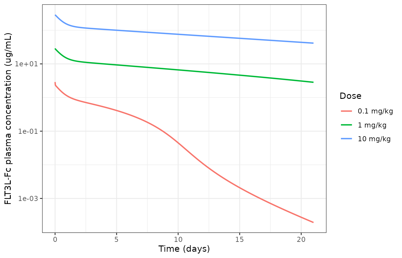
Replicates Figure 2A of Hosseini 2024: simulated single-dose FLT3L-Fc PK in cynomolgus monkeys.
Figure 3 of the paper shows the projected target expression and the three receptor-occupancy metrics. The paper’s key qualitative finding is that double-bound occupancy is not monotone in dose: it peaks at 0.1 mg/kg and falls away at higher doses, because excess free drug drives the equilibrium from the active homodimer towards the inactive single-bound complex.
cynoRo <- bind_rows(lapply(c(0.01, 0.03, 0.1, 1, 10), solveCyno)) |>
  mutate(treatment = factor(treatment,
                            levels = paste0(c(0.01, 0.03, 0.1, 1, 10), " mg/kg"))) |>
  select(time, treatment, RO, ROsb, ROdb) |>
  pivot_longer(c(RO, ROsb, ROdb), names_to = "metric", values_to = "pct") |>
  mutate(metric = recode(metric,
                         RO = "Total RO", ROsb = "Single-bound RO",
                         ROdb = "Double-bound RO"))

ggplot(cynoRo, aes(time / 24, pct, colour = treatment)) +
  geom_line(linewidth = 0.7) +
  facet_wrap(~metric) +
  labs(x = "Time (days)", y = "Receptor occupancy (%)", colour = "Dose") +
  theme_bw()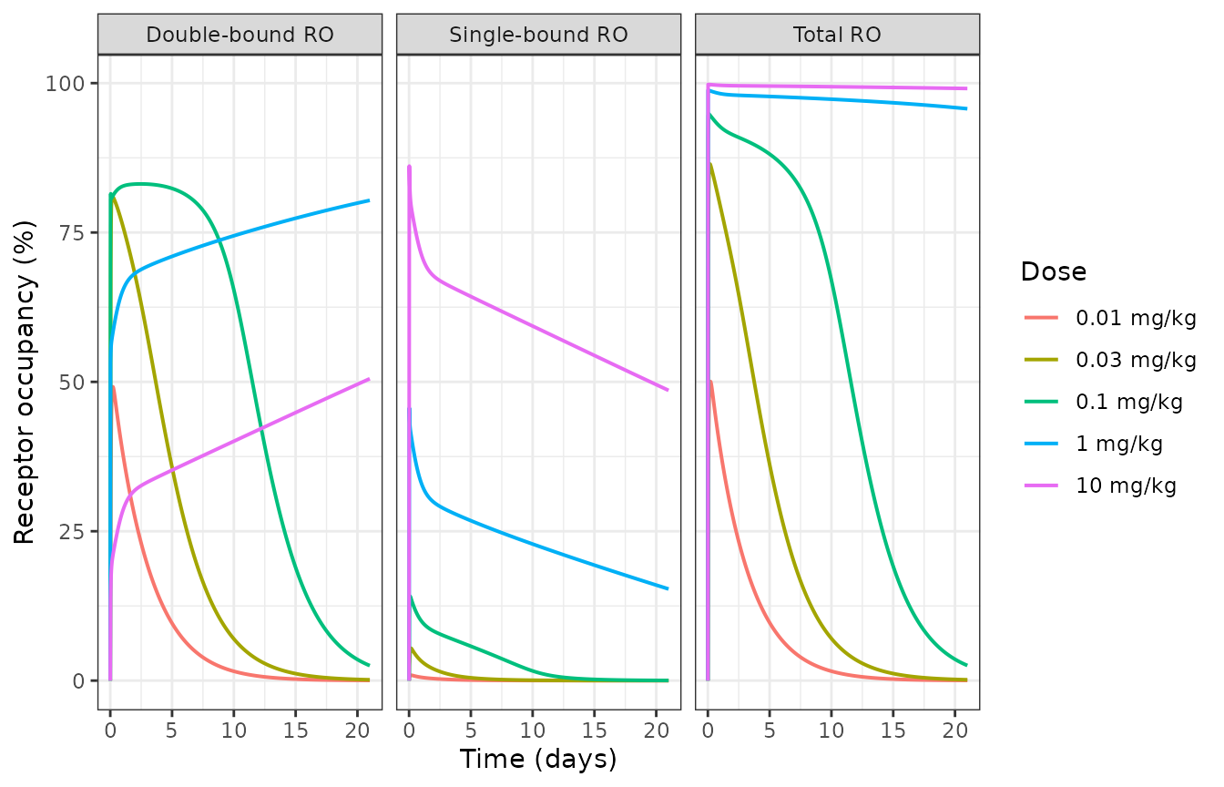
Replicates Figure 3B-D of Hosseini 2024: total, single-bound and double-bound FLT3 receptor occupancy after a single FLT3L-Fc dose in cynomolgus monkeys.
roPeak <-
  bind_rows(lapply(c(0.01, 0.03, 0.1, 1, 10), solveCyno)) |>
  group_by(dose_mgkg) |>
  summarise(maxROdb = max(ROdb), maxRO = max(RO), .groups = "drop")
knitr::kable(roPeak, digits = 1,
caption = "Peak receptor occupancy by dose (cynomolgus monkey).")| dose_mgkg | maxROdb | maxRO |
|---|---|---|
| 0.0 | 49.2 | 50.1 |
| 0.0 | 81.1 | 86.5 |
| 0.1 | 83.1 | 94.8 |
| 1.0 | 80.4 | 98.8 |
| 10.0 | 50.5 | 99.8 |
The paper states that double-bound occupancy “reached its peak at 0.1 mg/kg (83%) and declined following doses ranging from 1 to 10 mg/kg”, and that “at 1 mg/kg and higher, the model predicts near-complete receptor occupancy”.
peak01 <- roPeak$maxROdb[roPeak$dose_mgkg == 0.1]
stopifnot(
  # Published value: 83%.
  abs(peak01 - 83) < 3,
  # 0.1 mg/kg is the maximum of the double-bound curve across the dose range.
  which.max(roPeak$maxROdb) == which(roPeak$dose_mgkg == 0.1),
  # Double-bound occupancy declines monotonically from 1 to 10 mg/kg.
  all(diff(roPeak$maxROdb[roPeak$dose_mgkg >= 1]) < 0),
  # Near-complete total occupancy at 1 mg/kg and above.
  all(roPeak$maxRO[roPeak$dose_mgkg >= 1] > 98)
)
PKNCA validation against the published exposure summary
The paper reports observed AUC from days 0 to 21 and total clearance for the cynomolgus dose range: “AUC0-21 for 0.1 to 10 mg/kg ranged from 7 +/- 0.497 to 1660 +/- 336 ug/mL.day, and corresponding total clearance (CL) ranged from 13.7 +/- 0.901 to 4.92 +/- 1.96 mL/day/kg.”
ncaConc <-
  bind_rows(lapply(c(0.1, 10), solveCyno, days = 21, by = 0.25)) |>
  mutate(id = 1L) |>
  filter(!is.na(Cc)) |>
  select(id, treatment, time, Cc)

ncaDose <- data.frame(
  id        = 1L,
  treatment = c("0.1 mg/kg", "10 mg/kg"),
  time      = 0,
  amt       = c(0.1, 10) * 1000 * BW_CYNO
)

ncaObj <- PKNCA::PKNCAdata(
  PKNCA::PKNCAconc(ncaConc, Cc ~ time | treatment + id),
  PKNCA::PKNCAdose(ncaDose, amt ~ time | treatment + id,
                   route = "intravascular"),
  intervals = data.frame(
    start = 0, end = 21 * 24,
    auclast = TRUE, cmax = TRUE, tmax = TRUE
  )
)
ncaRes <- PKNCA::pk.nca(ncaObj, verbose = FALSE)

simNca <-
  as.data.frame(ncaRes) |>
  filter(PPTESTCD %in% c("auclast", "cmax", "tmax")) |>
  mutate(
    # AUC in ug/mL*h from the h-based time grid; the paper reports ug/mL*day.
    PPORRES = ifelse(PPTESTCD == "auclast", PPORRES / 24, PPORRES),
    PPORRES = ifelse(PPTESTCD == "tmax", PPORRES / 24, PPORRES)
  ) |>
  select(treatment, PPTESTCD, PPORRES)
refNca <- data.frame(
  treatment = c("0.1 mg/kg", "10 mg/kg"),
  auclast   = c(7, 1660)     # ug/mL*day, Hosseini 2024 Results section 3.2
)

cmpTbl <- nlmixr2lib::ncaComparisonTable(
  simNca, refNca,
  by     = "treatment",
  params = "auclast",
  units  = c(auclast = "ug/mL*day")
)
knitr::kable(cmpTbl, digits = 1,
caption = "Simulated vs published AUC(0-21 d) in cynomolgus monkeys.")| NCA parameter | treatment | Reference | Simulated | % diff |
|---|---|---|---|---|
| AUClast (ug/mL*day) | 0.1 mg/kg | 7 | 5.34 | -23.7%* |
| AUClast (ug/mL*day) | 10 mg/kg | 1660 | 1730 | +3.9% |
attr(cmpTbl, "footnote")
#> [1] "* differs from reference by more than ±20%."
clTbl <-
  simNca |>
  filter(PPTESTCD == "auclast") |>
  mutate(
    dose_ugkg     = c(100, 10000)[match(treatment, c("0.1 mg/kg", "10 mg/kg"))],
    CL_mL_day_kg  = dose_ugkg / PPORRES,
    published_CL  = c(13.7, 4.92)[match(treatment, c("0.1 mg/kg", "10 mg/kg"))]
  ) |>
  select(treatment, `AUC0-21 (ug/mL*day)` = PPORRES,
         `CL = dose/AUC (mL/day/kg)` = CL_mL_day_kg,
         `Published CL (mL/day/kg)` = published_CL)
knitr::kable(clTbl, digits = 2,
caption = "Dose-dependent clearance, simulated vs published.")| treatment | AUC0-21 (ug/mL*day) | CL = dose/AUC (mL/day/kg) | Published CL (mL/day/kg) |
|---|---|---|---|
| 0.1 mg/kg | 5.34 | 18.72 | 13.70 |
| 10 mg/kg | 1725.39 | 5.80 | 4.92 |
The simulated AUC at 10 mg/kg is within 5% of the observed mean. At 0.1 mg/kg the simulation is about 24% below the observed mean of 7 ug/mL.day — outside the 20% flag but consistent with the published Figure 2A fit, which is at its loosest at the lowest, most target-dominated dose. The values are not tuned to close this gap. Two features of the source explain it: the observed summary pools ADA-positive and ADA-negative samples while the model describes only ADA-negative disposition, and the reported clearances are not internally consistent with the reported AUC0-21 at the top dose either (10 000 / 1660 = 6.0 mL/day/kg against a reported 4.92), indicating that the published CL was computed over a longer window than the AUC0-21 it is tabulated beside.
What the model does reproduce exactly is the nonlinearity the paper draws its conclusions from:
Human: CDX-301 PK/PD calibration
The PD block was calibrated with the comparator molecule CDX-301,
whose PK is described empirically by a one-compartment SC model with
Michaelis-Menten elimination. fcflag = 0 selects CDX-301 as
the PD driver. CDX-301 amounts are body-weight normalised, so a 25 ug/kg
dose is entered as amt = 25 into depot.
solveCdx <- function(ugkg, days, horizon = 40) {
  ev <- rxode2::et(amt = ugkg, cmt = "depot", ii = 24, addl = days - 1)
  ev <- rxode2::et(ev, seq(0, horizon * 24, by = 1))
  out <- rxode2::rxSolve(modHuman, ev, params = c(fcflag = 0),
                         atol = 1e-10, rtol = 1e-8, returnType = "data.frame")
  out$treatment <- paste0(ugkg, " ug/kg x ", days, " d")
  out$ugkg <- ugkg
  out$days <- days
  out
}

study1 <- bind_rows(Map(solveCdx,
                        ugkg = c(3, 10, 25, 25, 75),
                        days = c(5, 5, 5, 10, 5)))
study2 <- bind_rows(Map(solveCdx,
                        ugkg = c(10, 25, 50, 75, 100),
                        days = rep(14, 5)))
ggplot(study1, aes(time / 24, Ccdx * 1000, colour = treatment)) +
  geom_line(linewidth = 0.7) +
  coord_cartesian(xlim = c(0, 15)) +
  labs(x = "Time (days)", y = "CDX-301 concentration (ng/mL)", colour = NULL) +
  theme_bw()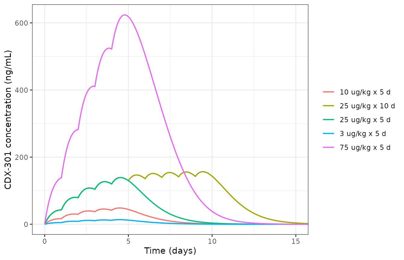
Replicates Figure 4A of Hosseini 2024: simulated CDX-301 PK after daily SC dosing in healthy volunteers.
ggplot(study1, aes(time / 24, cdc1, colour = treatment)) +
  geom_line(linewidth = 0.7) +
  geom_hline(yintercept = 1180, linetype = "dashed", colour = "grey40") +
  labs(x = "Time (days)", y = "cDC1 (cells/mL)", colour = NULL) +
  theme_bw()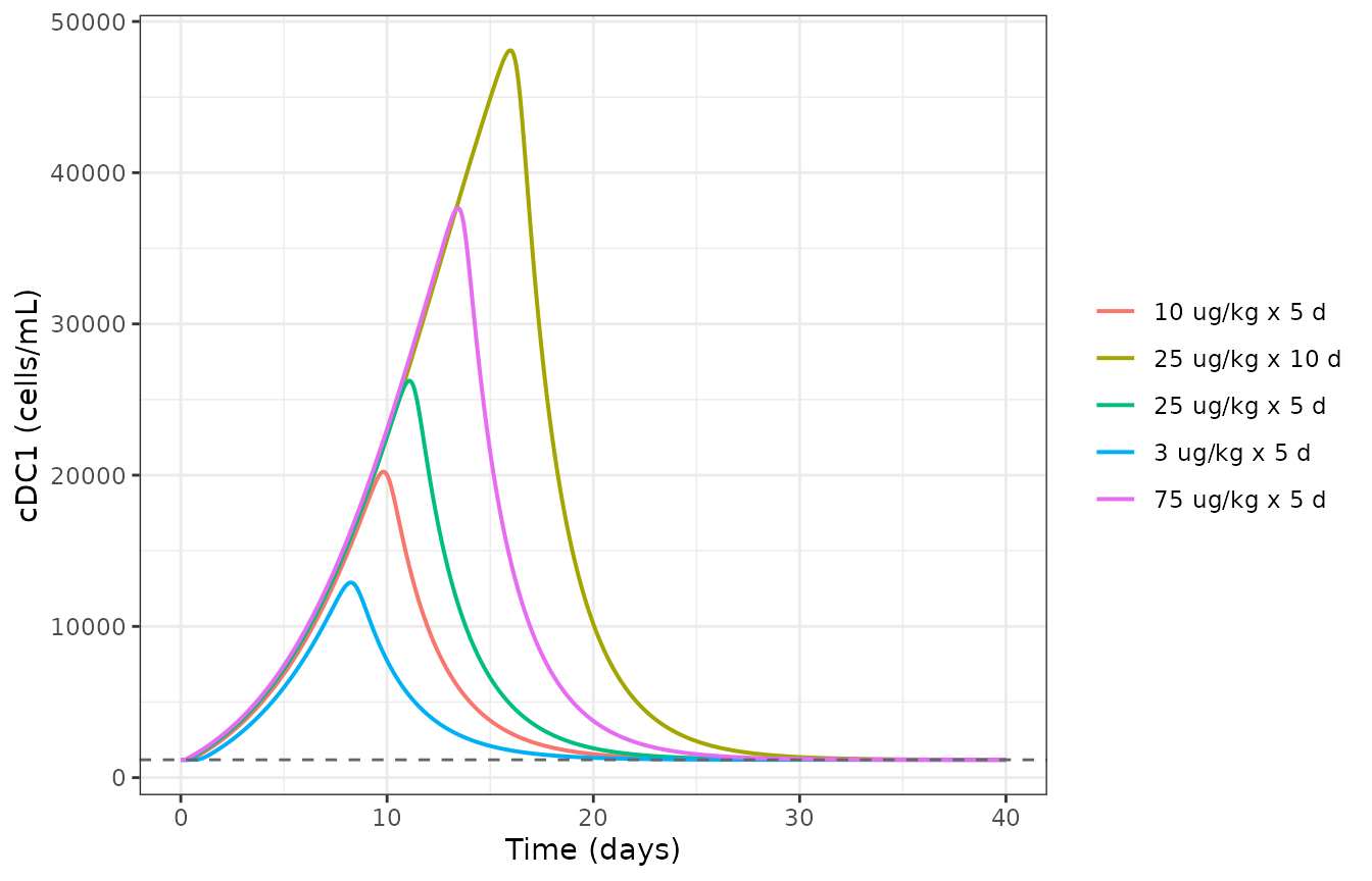
Replicates Figure 4B of Hosseini 2024: dose-dependent cDC1 expansion during and after daily CDX-301 dosing.
ggplot(study2, aes(time / 24, DCtotal, colour = treatment)) +
  geom_line(linewidth = 0.7) +
  labs(x = "Time (days)", y = "Total DC (cells/mL)", colour = NULL) +
  theme_bw()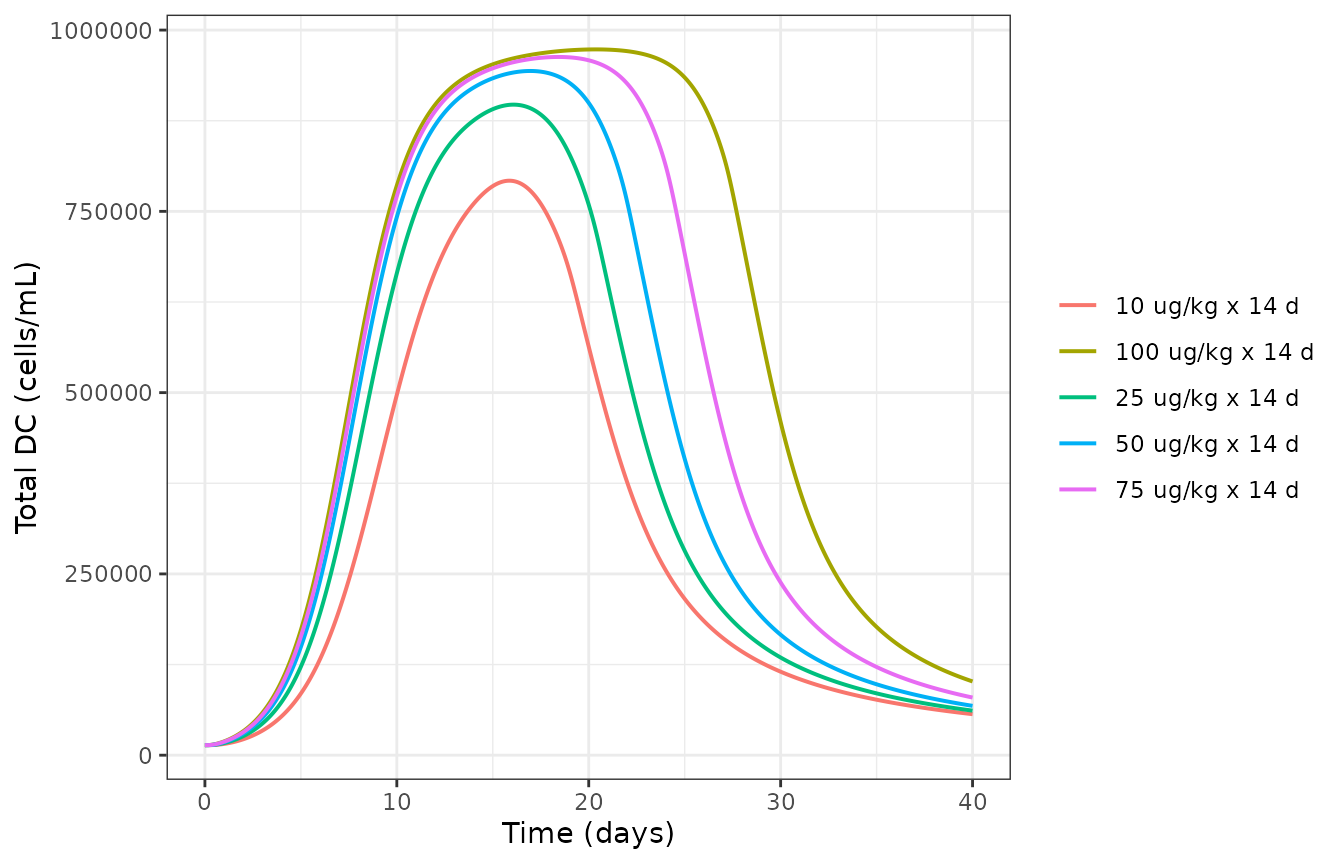
Replicates Figure 4C-D of Hosseini 2024: total DC expansion saturates between 10 and 100 ug/kg/day given for 14 days.
The paper’s validation claim for clinical study 2 is that “total DC expansion was comparable between the lowest dose (10 ug/kg/day) and the highest dose (100 ug/kg/day) following 14 days of daily treatments”, with saturation apparent around day 10.
peakStudy2 <-
  study2 |>
  group_by(ugkg) |>
  summarise(peakDCtotal = max(DCtotal), .groups = "drop")
knitr::kable(peakStudy2, digits = 0,
caption = "Peak total DC count after 14 days of daily recombinant FLT3L.")| ugkg | peakDCtotal |
|---|---|
| 10 | 792277 |
| 25 | 897163 |
| 50 | 943596 |
| 75 | 962921 |
| 100 | 973357 |
stopifnot(
  # Saturating, so still monotone in dose but far less than dose-proportional:
  # a 10-fold dose range must move peak total DC by less than 50%.
  all(diff(peakStudy2$peakDCtotal) > 0),
  max(peakStudy2$peakDCtotal) / min(peakStudy2$peakDCtotal) < 1.5,
  # Baseline is held exactly in the absence of drug.
  abs(study2$DCtotal[study2$time == 0][1] - (1180 + 12700)) < 1e-6
)
Human: FLT3L-Fc projections and the first-in-human dose
Switching fcflag = 1 drives the same PD block from free
FLT3L-Fc plasma concentration. Figure 6 of the paper projects PK, cDC1
and total DC for q3w IV dosing under two scenarios. Table S2’s human
column is the human-derived scenario, in which the FLT3
target parameters were refined against GS-3583 clinical PK; the
cyno-derived scenario substitutes the four cyno target
parameters.
CYNO_DERIVED <- c(fcflag = 1, rbase_target = 11.3, vmax_prolif = 1.90e-3,
                  km_prolif = 0.547, hill_prolif = 3.93)

solveFc <- function(dose_mgkg, params = c(fcflag = 1), cycles = 4) {
  ev <- rxode2::et(amt = dose_mgkg * 1000 * BW_HUMAN, cmt = "plasma",
                   ii = 21 * 24, addl = cycles - 1)
  ev <- rxode2::et(ev, seq(0, cycles * 21 * 24, by = 1))
  out <- rxode2::rxSolve(modHuman, ev, params = params,
                         atol = 1e-10, rtol = 1e-8, returnType = "data.frame")
  out$dose_mgkg <- dose_mgkg
  out$treatment <- paste0(dose_mgkg, " mg/kg")
  out
}

doses  <- c(0.01, 0.03, 0.1, 0.3, 1)
fcHum  <- bind_rows(lapply(doses, solveFc))
fcCyno <- bind_rows(lapply(doses, solveFc, params = CYNO_DERIVED))
fcHum |>
  select(time, treatment, Cc, cdc1, DCtotal) |>
  pivot_longer(c(Cc, cdc1, DCtotal), names_to = "output", values_to = "value") |>
  mutate(output = recode(output,
                         Cc = "FLT3L-Fc (ug/mL)",
                         cdc1 = "cDC1 (cells/mL)",
                         DCtotal = "Total DC (cells/mL)")) |>
  ggplot(aes(time / 24, value, colour = treatment)) +
  geom_line(linewidth = 0.7) +
  facet_wrap(~output, ncol = 1, scales = "free_y") +
  labs(x = "Time (days)", y = NULL, colour = "Dose") +
  theme_bw()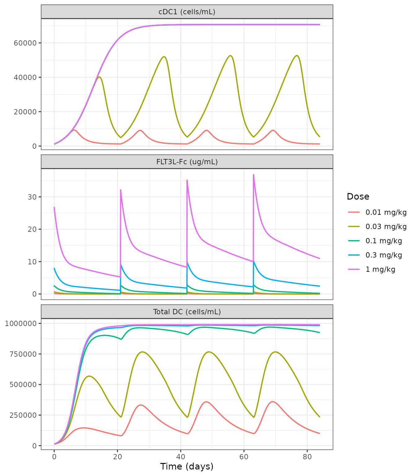
Replicates Figure 6 of Hosseini 2024: projected FLT3L-Fc PK, cDC1 and total DC for q3w IV dosing under the human-derived scenario.
cycle1 <- fcHum |> filter(dose_mgkg == 0.01, time <= 21 * 24)

fih <- tibble(
  Quantity = c("Peak cDC1 (cells/mL)", "cDC1 fold expansion",
               "Maximum total RO (%)", "Mean total RO over 21 days (%)"),
  Simulated = c(max(cycle1$cdc1), max(cycle1$cdc1) / 1180,
                max(cycle1$RO), mean(cycle1$RO)),
  Published = c(9500, 8, 67, 16)
)
knitr::kable(fih, digits = c(0, 1, 1, 1),
caption = "First-in-human dose (700 ug = 0.01 mg/kg IV): simulated vs published.")| Quantity | Simulated | Published |
|---|---|---|
| Peak cDC1 (cells/mL) | 9326.7 | 9500 |
| cDC1 fold expansion | 7.9 | 8 |
| Maximum total RO (%) | 66.7 | 67 |
| Mean total RO over 21 days (%) | 15.9 | 16 |
stopifnot(
  # Published: peak peripheral blood cDC1 of 9500 cells/mL, about 8-fold.
  abs(max(cycle1$cdc1) - 9500) / 9500 < 0.10,
  abs(max(cycle1$cdc1) / 1180 - 8) < 0.8,
  # Published: maximum total RO 67%, average RO over 21 days about 16%.
  abs(max(cycle1$RO) - 67) < 3,
  abs(mean(cycle1$RO) - 16) < 2
)
The paper also states that the human-derived scenario maximises DC expansion at 0.1 mg/kg, that the cyno-derived scenario needs “about a three-fold greater dose” (0.3 mg/kg) to do the same, and that cDC1 and total DC plateau near 70 000 and 1 000 000 cells/mL respectively.
plateau <-
  bind_rows(
    fcHum  |> mutate(scenario = "Human-derived"),
    fcCyno |> mutate(scenario = "Cyno-derived")
  ) |>
  group_by(scenario, dose_mgkg) |>
  summarise(peak_cDC1 = max(cdc1), peak_DCtotal = max(DCtotal),
            .groups = "drop") |>
  arrange(desc(scenario), dose_mgkg)
knitr::kable(plateau, digits = 0,
caption = "Peak cDC1 and total DC by dose under both target-parameter scenarios.")| scenario | dose_mgkg | peak_cDC1 | peak_DCtotal |
|---|---|---|---|
| Human-derived | 0 | 9327 | 359814 |
| Human-derived | 0 | 52595 | 766599 |
| Human-derived | 0 | 70630 | 969474 |
| Human-derived | 0 | 70630 | 986558 |
| Human-derived | 1 | 70630 | 990564 |
| Cyno-derived | 0 | 2696 | 64963 |
| Cyno-derived | 0 | 7723 | 413817 |
| Cyno-derived | 0 | 53740 | 864824 |
| Cyno-derived | 0 | 70630 | 984080 |
| Cyno-derived | 1 | 70630 | 990408 |
maxCdc1 <- max(plateau$peak_cDC1)
hum <- plateau |> filter(scenario == "Human-derived")
cyn <- plateau |> filter(scenario == "Cyno-derived")

# Lowest dose reaching 95% of the achievable plateau, in each scenario.
minDoseAt95 <- function(x) min(x$dose_mgkg[x$peak_cDC1 >= 0.95 * maxCdc1])

stopifnot(
  # Published plateaus: cDC1 ~70,000 and total DC ~1,000,000 cells/mL.
  abs(maxCdc1 - 70000) / 70000 < 0.10,
  abs(max(plateau$peak_DCtotal) - 1e6) / 1e6 < 0.10,
  # Published: 0.1 mg/kg (human-derived) vs 0.3 mg/kg (cyno-derived), 3-fold.
  minDoseAt95(hum) == 0.1,
  minDoseAt95(cyn) == 0.3,
  # The FIH dose sits below 20% of maximal cDC1 expansion, the stated criterion.
  max(cycle1$cdc1) / maxCdc1 < 0.20
)
Assumptions and deviations
Errata and source conflicts
-
Manuscript Eq 4 has a transcription error. It
writes
dCRpR/dt = kon2*Cp*CRp - koff2*CRpR - kdeg*CRpR, i.e. the double-bound complex forming from free drug plus the single-bound complex. Eq 3 writes the matching loss term as-kon2*CR*CRp(free receptor plus the single-bound complex), and the supplement’s SimBiology export confirms Eq 3:kon2_1nMh*Complex_SB_Central_nM*TargetCentral_nM. The mechanism requires the latter — a homodimer is one drug bridging two receptors — and only the latter conserves drug mass, which is why the plasma ODE carries nokon2term. The models encode the supplement form. -
km_prolifis on the fraction scale, not the percentage scale. The manuscript calls it “the percentage of FLT3 RODB to achieve 50% of maximum expansion”, but the supplement ODE compares it againstRO_DB/100. Read as a percentage, the cyno value 0.547 would mean half-maximal expansion at 0.5% occupancy and the model would not reproduce Figure 3. -
Two Table S2 unit labels are wrong.
ISFis captionedmL/kg, but the SimBiology project names the parameterISF_Land consumes it as a volume in litres; 15.6 L is the Cao 2013 whole-body interstitial volume and 0.579 L is its cynomolgus counterpart.vmCDXis captionedmL/h/kgbut the supplement names the parameterVm_CDX_ughkgand uses it as an amount rate; only ug/h/kg is dimensionally consistent withVm*C/(Km+C)whereCandKmshare units. -
The tissue partition is sourced from the SimBiology project,
not Table S2. Table S2 reports
fleaky = 0.65andftight = 0.35under flow-fraction captions, but those numbers are the interstitial volume split. The supplement’s SimBiology project settles it directly: it stores the four assignments verbatim asVtight_L = 0.65*ISF_L*Kp,Vleaky_L = 0.35*ISF_L*Kp,L_tight_Lh = 0.33*L_LhandL_leaky_Lh = 0.67*L_Lh. That is the standard Cao 2013 mPBPK convention (tight tissues hold 65% of the interstitial volume but receive 33% of lymph flow) and is whatYuan_2019_concizumabalready uses in this package. The models reproduce those four formulas and apply them to the cynomolgus system parameters as well.
Deviations from the SimBiology model
-
Tissue-level target binding is omitted. The
SimBiology export carries
TargetTight,TargetLeaky,ComplexTightandComplexLeakystates, but Table S2 reports no synthesis, degradation or baseline values for them and the manuscript is explicit that TMDD is in the central compartment only (Section 2.4, Figure 1A). Those states are inactive in the published parameterisation, so the models carry only the plasma target and complexes and describe tissue distribution by convection alone, as manuscript Eq 1 does. -
IV dosing goes directly into
plasma. The SimBiology export routes the IV dose through a first-order transfer state (infusion_Fc_ug) governed byinf_time_h, which is not reported anywhere in the paper (the project file’s default is 1 h). Rather than adopt an unreported value, the models let rxode2 handle IV administration natively; users who want a finite infusion can supplyrateorduron the dose row of the event table. -
A linear
CL_CDXterm is omitted. The SimBiology CDX-301 ODE contains a first-order clearance term alongside the Michaelis-Menten term, but Table S2 reports no value for it and both the manuscript equation and its prose describe nonlinear elimination only, so it is zero in the published model. -
The CDX-301 cross-feed into the FLT3L-Fc plasma compartment
is omitted. The SimBiology
d(AmtCentral_ug)/dtcarries a+ kabs_CDX*SCdepot_CDX_ugterm, fed by a second, non-weight-normalised CDX depot state (SCdepot_CDX_ug) that exists alongside theSCdepot_CDX_ugkgstate the CDX-301 sub-model actually uses. It lets one configuration of the project push CDX-301 through the Fc disposition block instead of its own empirical one. Every CDX-301 result in the paper is generated from the ug/kg depot, so that state is never dosed and the term is identically zero; the models carry only the ug/kg depot. -
C3is a flooredC2, not a third transit state. The manuscript calls the PD driver “the drug-concentration in the third transit compartment”, but the supplement has only two transit ODEs per cell type and definesC3_DCx = max(C2_DCx, 1e-6). The models replicate the supplement. -
Numerical guards.
max(target_tot, 1e-18)in the occupancy denominators and themax(., 1e-6)floor on the transit signal are taken from the supplement’s own repeated assignments. The additionalmax(ro_db/100, 0)before the Hill power is an equivalent guard against solver round-off producing a negative base under a fractional exponent; it is inactive whenever the state is physically valid.
Scope
- No variability. The paper reports no IIV, no residual error and no parameter uncertainty, so none is encoded. These models simulate typical profiles; they are not fit-ready population models.
- ADA is not described. Anti-drug antibodies were detected in every cynomolgus monkey by day 14 and reduced late exposure, but the authors deliberately excluded ADA from the model because nonclinical immunogenicity translates poorly. Simulated late-phase cynomolgus concentrations therefore correspond to ADA-negative samples and will overpredict ADA-positive ones.
- The PD arm was fitted to digitized group means from two published CDX-301 / recombinant FLT3L studies, not to individual-subject data, and FLT3L-Fc and CDX-301 are assumed equipotent per nanomolar on cDC expansion.
- Both target-parameter scenarios are reachable. The human model ships the human-derived scenario (Table S2 human column). The cyno-derived scenario is obtained by overriding four parameters, as shown above; it is a parameter variant of the same structure, not a separate published model.