Intravenous immunoglobulin in Guillain-Barre syndrome (Fokkink 2022)
Source:vignettes/articles/Fokkink_2022_immunoglobulin.Rmd
Fokkink_2022_immunoglobulin.RmdModel and source
- Citation: Fokkink WJR, van Tilburg SJ, de Winter BCM, Sassen SDT, van Doorn PA, Koch BCP, Jacobs BC. Population pharmacokinetic modelling of intravenous immunoglobulin treatment in patients with Guillain-Barre syndrome. Clin Pharmacokinet. 2022;61(9):1285-1296. doi:10.1007/s40262-022-01136-z
- Description: Two-compartment population PK model for high-dose intravenous immunoglobulin (IVIg) in Guillain-Barre syndrome, fitted to total serum IgG (IVIg-derived plus an estimated endogenous baseline) with allometric weight scaling and disease-severity (GBS disability score) and concomitant methylprednisolone effects on clearance (Fokkink 2022)
- Article: https://doi.org/10.1007/s40262-022-01136-z (open access; the Electronic Supplementary Material contains the final NONMEM control stream)
Population
The model-building cohort combined 177 patients with Guillain-Barre syndrome (GBS) from two Dutch GBS Study Group randomised trials – IVIg versus plasma exchange, and IVIg with or without intravenous methylprednisolone (500 mg/day for 5 days) – with 15 patients with stable chronic inflammatory demyelinating polyneuropathy (CIDP) on IVIg maintenance, who supplied samples shortly after infusion. GBS patients were unable to walk independently at entry and all received IVIg 0.4 g/kg/day for 5 consecutive days (Gammagard S/D). The GBS cohort (Fokkink 2022 Table 1) had mean age 53 years (range 5-89), mean weight 72 kg (range 18-122), 57% male, mean GBS disability score (GBS-DS) 4.1 at nadir, 25% mechanically ventilated and 34% treated with methylprednisolone. Total serum IgG was measured by turbidimetry (589 GBS samples, 222 CIDP samples). The model was externally validated in 177 good-prognosis patients of the SID-GBS trial.
The same information is available programmatically via
readModelDb("Fokkink_2022_immunoglobulin")()$population.
Source trace
The per-parameter origin is recorded as an in-file comment next to
each ini() entry in
inst/modeldb/specificDrugs/Fokkink_2022_immunoglobulin.R.
| Equation / parameter | Value | Source location |
|---|---|---|
| Two-compartment IV model, elimination from central | – | Results 3.1.1; Fig. 1; ESM control stream
ADVAN3 TRANS4
|
| Total IgG = IVIg-derived + CBAS | – | Methods 2.3.1; ESM $ERROR
FTOT = F + CBAS
|
lcl (CL, L/day per 70 kg) |
0.28 | Table 2, final model |
lvc (V1, L) |
2.87 | Table 2, final model |
lq (Q, L/day) |
0.25 | Table 2, final model |
lvp (V2, L) |
2.65 | Table 2, final model |
e_wt_cl_q |
0.75 (fixed) | Results 3.1.1; ESM THETA(6) FIX |
e_wt_vc_vp |
1 (fixed) | Results 3.1.1; ESM THETA(7) FIX |
lbl_igg (CBAS, g/L, CIDP) |
15.90 | Table 2, final model |
e_dis_gbs_bl_igg |
0.65 | Table 2 ‘Disease type (if GBS)’; Methods 2.3.1 equation |
e_conmed_methylprednisolone_cl |
1.31 | Table 2; Results 3.1.2 |
e_score_gbs_disability_34_cl |
1.22 | Table 2; Results 3.1.2 |
e_score_gbs_disability_5_cl |
1.83 | Table 2; Results 3.1.2 |
| GBS-DS grouping 0-2 / 3-4 / 5 | – | Results 3.1.2; ESM FSCORE block |
etalcl |
49.9% CV | Table 2 IIV |
etalbl_igg |
23.1% CV | Table 2 IIV |
propSd |
0.12 | Table 2 residual error; ESM $ERROR
|
Simulation of the paper’s Figure 4 scenarios
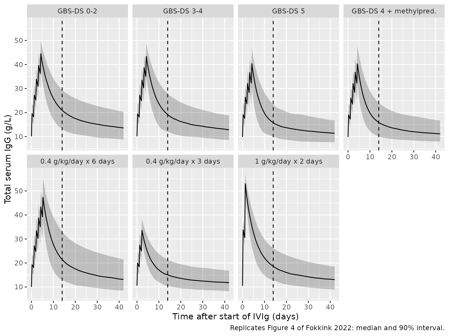
Figure 4 of the paper simulates a 75 kg patient with GBS receiving 0.4 g/kg IVIg as a 2-hour infusion each day for 5 days. The reference scenario is a GBS-DS of 4 without methylprednisolone; panels B-D vary the disability score, add methylprednisolone, and change the regimen. Each scenario below has 200 virtual patients with between-subject variability on CL and baseline IgG.
mod <- readModelDb("Fokkink_2022_immunoglobulin")

scenarios <- tibble::tribble(
  ~scenario,                  ~score, ~mp, ~ndays, ~dose_kg,
  "GBS-DS 0-2",                   2,   0,      5,      0.4,
  "GBS-DS 3-4",                   4,   0,      5,      0.4,
  "GBS-DS 5",                     5,   0,      5,      0.4,
  "GBS-DS 4 + methylpred.",       4,   1,      5,      0.4,
  "0.4 g/kg/day x 6 days",        4,   0,      6,      0.4,
  "0.4 g/kg/day x 3 days",        4,   0,      3,      0.4,
  "1 g/kg/day x 2 days",          4,   0,      2,      1.0
) |>
  mutate(scenario = factor(scenario, levels = scenario))

n_per_arm <- 200
wt <- 75
obs_times <- sort(unique(c(seq(0, 7, by = 0.25), seq(7, 42, by = 1))))

make_arm <- function(i) {
  s <- scenarios[i, ]
  ids <- (i - 1) * n_per_arm + seq_len(n_per_arm)
  dose <- expand.grid(id = ids, day = seq_len(s$ndays) - 1) |>
    transmute(
      id, time = day, amt = s$dose_kg * wt, rate = s$dose_kg * wt / (2 / 24),
      evid = 1L, cmt = "central"
    )
  obs <- expand.grid(id = ids, time = obs_times) |>
    mutate(amt = 0, rate = 0, evid = 0L, cmt = "central")
  bind_rows(dose, obs) |>
    mutate(
      scenario = s$scenario, WT = wt, SCORE_GBS_DISABILITY = s$score,
      CONMED_METHYLPREDNISOLONE = s$mp, DIS_GBS = 1L
    )
}
events <- bind_rows(lapply(seq_len(nrow(scenarios)), make_arm)) |>
  arrange(id, time, desc(evid))

rxode2::rxSetSeed(20220704)
sim <- rxode2::rxSolve(
  mod, events,
  keep = "scenario", returnType = "data.frame"
) |>
  mutate(delta_igg = Cc - bl_igg)
#> ℹ parameter labels from comments will be replaced by 'label()'
sim |>
  group_by(scenario, time) |>
  summarise(
    med = median(Cc), lo = quantile(Cc, 0.05), hi = quantile(Cc, 0.95),
    .groups = "drop"
  ) |>
  ggplot(aes(time, med)) +
  geom_ribbon(aes(ymin = lo, ymax = hi), alpha = 0.25) +
  geom_line() +
  geom_vline(xintercept = 14, linetype = "dashed") +
  facet_wrap(~scenario, ncol = 4) +
  labs(
    x = "Time after start of IVIg (days)", y = "Total serum IgG (g/L)",
    caption = "Replicates Figure 4 of Fokkink 2022: median and 90% interval."
  )
Target attainment at two weeks
The paper’s pharmacodynamic target is an increase of total IgG over
baseline (delta IgG) above 7.3 g/L at 2 weeks. In this model delta IgG
is the IVIg-derived concentration central / vc, so the
baseline cancels and only the clearance random effect matters. Because
delta IgG at day 14 falls monotonically as clearance rises, the
attainment probability is exact: find the etalcl at which a
typical patient sits on the 7.3 g/L target, then evaluate the normal
distribution function at that threshold. This gives a reference that
does not depend on the random seed. The 200-patient simulation from the
previous section is shown next to it.
ui <- suppressMessages(rxode2::rxode(mod))
typ <- suppressMessages(rxode2::zeroRe(ui))
omega_cl <- sqrt(ui$omega["etalcl", "etalcl"])
lcl0 <- ui$theta[["lcl"]]

delta_day14 <- function(eta, score, mp, ndays, dose_kg) {
  ev <- data.frame(
    id = 1, time = c(seq_len(ndays) - 1, 14),
    amt = c(rep(dose_kg * wt, ndays), 0),
    rate = c(rep(dose_kg * wt / (2 / 24), ndays), 0),
    evid = c(rep(1L, ndays), 0L), cmt = "central",
    WT = wt, SCORE_GBS_DISABILITY = score,
    CONMED_METHYLPREDNISOLONE = mp, DIS_GBS = 1L
  )
  s <- suppressMessages(rxode2::rxSolve(
    typ, ev,
    params = c(lcl = lcl0 + eta), returnType = "data.frame"
  ))
  s$Cc[s$time == 14] - s$bl_igg[s$time == 14]
}

exact_pta <- vapply(seq_len(nrow(scenarios)), function(i) {
  s <- scenarios[i, ]
  eta_star <- uniroot(
    function(e) delta_day14(e, s$score, s$mp, s$ndays, s$dose_kg) - 7.3,
    c(-3, 3)
  )$root
  100 * pnorm(eta_star / omega_cl)
}, numeric(1))

sim_pta <- sim |>
  filter(time == 14) |>
  group_by(scenario) |>
  summarise(sim = 100 * mean(delta_igg > 7.3), .groups = "drop")

pta <- scenarios |>
  select(scenario) |>
  mutate(
    published = c(74, 63, 33, 43, 74, 12, 54),
    exact = exact_pta
  ) |>
  left_join(sim_pta, by = "scenario") |>
  mutate(diff = exact - published)

pta |>
  mutate(across(c(exact, sim, diff), \(x) round(x, 1))) |>
  dplyr::rename(
    "Scenario" = scenario,
    "Published (%)" = published,
    "Model, exact (%)" = exact,
    "Model, 200 simulated (%)" = sim,
    "Exact - published (points)" = diff
  ) |>
knitr::kable(caption = "Probability of delta IgG > 7.3 g/L at day 14 (Fokkink 2022 Results 3.2 and Figure 4).")| Scenario | Published (%) | Model, exact (%) | Model, 200 simulated (%) | Exact - published (points) |
|---|---|---|---|---|
| GBS-DS 0-2 | 74 | 78.2 | 74.5 | 4.2 |
| GBS-DS 3-4 | 63 | 63.9 | 60.0 | 0.9 |
| GBS-DS 5 | 33 | 30.6 | 33.5 | -2.4 |
| GBS-DS 4 + methylpred. | 43 | 41.4 | 33.5 | -1.6 |
| 0.4 g/kg/day x 6 days | 74 | 77.2 | 76.5 | 3.2 |
| 0.4 g/kg/day x 3 days | 12 | 18.4 | 17.5 | 6.4 |
| 1 g/kg/day x 2 days | 54 | 54.3 | 55.5 | 0.3 |
# The exact column is deterministic (no random draws), so a tight bound holds
# across rxode2 builds. The covariate ordering checks the direction of the
# GBS-DS and methylprednisolone effects and the regimen ranking.
stopifnot(
  all(abs(pta$diff) < 8),
  pta$exact[1] > pta$exact[2], pta$exact[2] > pta$exact[3],
  pta$exact[4] < pta$exact[2],
  pta$exact[5] > pta$exact[7], pta$exact[7] > pta$exact[6]
)
The exact attainment probabilities land within 5 percentage points of the paper’s Monte Carlo values (n = 1000 per scenario) for six of the seven scenarios, and every covariate and regimen effect points the same way. The largest gap is the 3-day regimen (about 18% versus the published 12%); the paper does not say whether its simulated delta IgG included residual error or how the baseline was subtracted, which matters most for a regimen whose typical patient sits just below the target.
Non-compartmental analysis
The paper reports no NCA. For completeness, PKNCA is run on the IVIg-derived concentration (total IgG minus the individual endogenous baseline) for the standard 5-day regimen in each GBS-DS group, over the 42-day simulation.
nca_conc <- sim |>
  filter(scenario %in% c("GBS-DS 0-2", "GBS-DS 3-4", "GBS-DS 5")) |>
  filter(!is.na(delta_igg)) |>
  transmute(id, time, conc = delta_igg, treatment = as.character(scenario))

nca_dose <- events |>
  filter(evid == 1, scenario %in% c("GBS-DS 0-2", "GBS-DS 3-4", "GBS-DS 5")) |>
  transmute(id, time, amt, treatment = as.character(scenario))

conc_obj <- PKNCA::PKNCAconc(nca_conc, conc ~ time | treatment + id)
dose_obj <- PKNCA::PKNCAdose(nca_dose, amt ~ time | treatment + id)
intervals <- data.frame(
  start = 0, end = 42,
  cmax = TRUE, tmax = TRUE, auclast = TRUE, half.life = TRUE
)
nca_res <- PKNCA::pk.nca(PKNCA::PKNCAdata(conc_obj, dose_obj, intervals = intervals))

nca_summary <- as.data.frame(nca_res$result) |>
  filter(PPTESTCD %in% c("cmax", "tmax", "auclast", "half.life")) |>
  group_by(treatment, PPTESTCD) |>
  summarise(median = signif(median(PPORRES, na.rm = TRUE), 3), .groups = "drop") |>
  tidyr::pivot_wider(names_from = PPTESTCD, values_from = median)

nca_summary |>
  dplyr::rename(
    "GBS-DS group" = treatment,
    "Cmax (g/L)" = cmax,
    "Tmax (day)" = tmax,
    "AUC0-42 (g*day/L)" = auclast,
    "t1/2 (day)" = half.life
  ) |>
knitr::kable(caption = "Median NCA of IVIg-derived IgG, 0.4 g/kg/day x 5 days, 75 kg.")| GBS-DS group | AUC0-42 (g*day/L) | Cmax (g/L) | t1/2 (day) | Tmax (day) |
|---|---|---|---|---|
| GBS-DS 0-2 | 424 | 34.5 | 18.0 | 4.25 |
| GBS-DS 3-4 | 360 | 33.1 | 15.6 | 4.25 |
| GBS-DS 5 | 262 | 30.1 | 12.7 | 4.25 |
Clearance rises with disease severity, so AUC falls from the 0-2 group to the GBS-DS 5 group while Cmax, which is governed by the central volume, changes much less.
Assumptions and deviations
-
CIDP clearance factor not encoded. The control
stream in the Electronic Supplementary Material estimates a separate
multiplicative factor on CL for the CIDP patients
(
THETA(10), GBS-DS coded -99), but the paper does not report its value. The model therefore applies the reference clearance to CIDP subjects (DIS_GBS = 0withSCORE_GBS_DISABILITYin 0-2). The CIDP baseline IgG (15.9 g/L) is reported and encoded. The model is intended for GBS; CIDP predictions of clearance are not supported by the paper. -
IIV covariance not encoded. The control stream uses
an
OMEGA BLOCK(2)on CL and CBAS, but only the two variances are reported, so the etas are independent. - IIV scale. Table 2 reports IIV as a percentage, which is read as a CV: omega^2 = log(1 + CV^2). The target-attainment comparison above does not separate this from omega = CV (the two differ by about 6% on the SD scale).
-
GBS-DS grouping. The score enters as the raw 0-6
value and is grouped in
model()exactly as the paper and control stream group it. A score of 6 (death) was disregarded by the authors and receives no CL factor. - Time units. The control stream ran in hours; Table 2 reports CL and Q in L/day, so the model runs in days.
-
Peripheral compartment.
peripheral1carries the IVIg-derived IgG distributing outside the central (vascular) space; the paper does not identify the tissue.