Model and source
- Citation: Kim W, Won JY, Yi J, Choi SC, Lee SM, Mun K, Lim HS. PK Modeling of L-4-Boronophenylalanine and Development of Bayesian Predictive Platform for L-4-Boronophenylalanine PKs for Boron Neutron Capture Therapy. Pharmaceuticals (Basel). 2024;17(3):301. doi:10.3390/ph17030301.
- Description: Two-compartment population PK model for whole-blood boron-10 after intravenous infusion of borofalan (10B) (L-4-boronophenylalanine, BPA, given as the BPA-fructose complex) in cancer patients undergoing boron neutron capture therapy. Fitted in NONMEM 7.4.3 (ADVAN13, FOCE-I) to 377 blood boron concentrations from 27 patients, digitised by the authors from seven published clinical reports. Parameterised in micro-constant form exactly as the authors report it (V1, k10, k12, k21) with log-normal IIV on all four and a combined additive + proportional residual error. Dosing and volume are per kilogram of body weight: the dose is mg/kg of BPA, V1 is L/kg, and the model converts the BPA amount to boron-10 with the authors’ factor 10/208.21, so the output is the boron-10 concentration in ug/g (ppm). The paper uses this model as the prior for Bayesian (MAP) prediction of the blood boron level during neutron irradiation.
- Article: https://doi.org/10.3390/ph17030301
L-4-[10B]boronophenylalanine (BPA; INN borofalan (10B)) is the boron carrier used in boron neutron capture therapy (BNCT). The radiation dose delivered during neutron irradiation depends on the boron-10 concentration in blood and tissue at the time of irradiation, and blood cannot be sampled while the patient is in the irradiation room. Kim et al. built a population PK model of whole-blood boron-10 after an intravenous BPA infusion and used it as the prior for Bayesian (MAP) prediction of the mean blood boron level during the irradiation window.
Population
The model was fitted to 377 whole-blood boron-10 concentrations from 27 cancer patients given an intravenous infusion of 10B-enriched BPA (as the BPA-fructose complex). No new clinical data were collected: the concentration-time points were digitised by the authors from seven published clinical reports (Kim 2024 references 8 and 10-15), which cover glioma / glioblastoma, malignant melanoma and head and neck cancer patients treated in Finland, the USA, China, an EORTC trial and Japan. Doses and infusion durations differ between the source reports (Figure 2 shows 250 mg/kg over 65 min and 290 mg/kg over 120 min); the paper’s own simulations use 500 mg/kg over 180 min. No demographics or covariates were available to the authors, and the final model has none (Kim 2024 Methods 2.1).
The same information is available programmatically via
rxode2::rxode(readModelDb("Kim_2024_borofalan"))$population.
Source trace
The per-parameter origin is recorded as an in-file comment next to
each ini() entry in
inst/modeldb/specificDrugs/Kim_2024_borofalan.R.
| Equation / parameter | Value | Source location |
|---|---|---|
lkel (K10) |
log(0.006) 1/min | Table 2 |
lk12 (K12) |
log(0.023) 1/min | Table 2 |
lk21 (K21) |
log(0.012) 1/min | Table 2 |
lvc (V1) |
log(0.252) L/kg | Table 2 (printed “L”; per-kg per Figure 4A, see below) |
etalkel |
0.050 (CV 22.6%) | Table 2, IIV K10 |
etalk12 |
0.071 (CV 27.2%) | Table 2, IIV K12 |
etalk21 |
0.037 (CV 19.4%) | Table 2, IIV K21 |
etalvc |
0.061 (CV 25.0%) | Table 2, IIV V1 |
addSd |
sqrt(0.540) ug/g | Table 2, eps1 (additive) |
propSd |
sqrt(0.001) | Table 2, eps2 (proportional) |
Individual parameters P_i = P_TV * exp(eta)
|
n/a | Methods 2.1 |
| Two-compartment linear disposition | n/a | Results 3.1 |
Boron-10 / BPA factor 10/208.21
|
n/a | Methods 2.1 |
Cobs = Cpred + eps1 + eps2 * Cpred |
n/a | Results 3.1 |
mod <- readModelDb("Kim_2024_borofalan")
ui <- rxode2::rxode(mod)
#> ℹ parameter labels from comments will be replaced by 'label()'
mod_typical <- rxode2::zeroRe(mod)
#> ℹ parameter labels from comments will be replaced by 'label()'
Unit check against Figure 4A (deterministic)
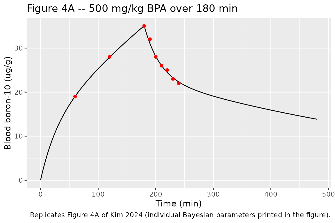
Figure 4A of the paper shows the platform’s Bayesian fit for a
simulated patient given 500 mg/kg BPA over 180 min, and prints that
patient’s individual parameters (K1 = 0.021817 1/min,
K2 = 0.01085 1/min, K3 = 0.0059167 1/min,
V1 = 0.22902 l/kg) together with the nine blood boron-10
values the fit was conditioned on. Solving the packaged model with those
individual parameters must reproduce the printed values. This pins the
per-kilogram volume, the mg/kg dosing unit and the 10/208.21 boron-10
conversion together: getting any one of them wrong moves the curve by a
factor of 70 (body weight) or 21 (the conversion), not by a few
percent.
fig4a <- tibble::tribble(
  ~time, ~published,
  60, 18.999,
  120, 27.999,
  180, 34.999,
  190, 31.999,
  200, 27.999,
  210, 25.999,
  220, 24.999,
  230, 22.999,
  240, 21.999
)

ev_fig4a <- rxode2::et(amt = 500, rate = 500 / 180, cmt = "central") |>
  rxode2::et(seq(0, 480, by = 2))

sim_fig4a <- rxode2::rxSolve(
  mod_typical,
  events = ev_fig4a,
  params = c(
    lk12 = log(0.021817),
    lk21 = log(0.01085),
    lkel = log(0.0059167),
    lvc = log(0.22902)
  )
) |>
  as.data.frame()
#> ℹ omega/sigma items treated as zero: 'etalkel', 'etalk12', 'etalk21', 'etalvc'

chk_fig4a <- fig4a |>
  dplyr::left_join(dplyr::select(sim_fig4a, time, Cc), by = "time") |>
  dplyr::mutate(pct_diff = 100 * (Cc - published) / published)

knitr::kable(
  chk_fig4a |>
    dplyr::rename(
      "Time (min)" = time,
      "Figure 4A (ug/g)" = published,
      "Packaged model (ug/g)" = Cc,
      "Difference (%)" = pct_diff
    ),
  digits = 2,
  caption = "Blood boron-10 at the Figure 4A sampling times, solved with the printed individual parameters."
)| Time (min) | Figure 4A (ug/g) | Packaged model (ug/g) | Difference (%) |
|---|---|---|---|
| 60 | 19 | 19.04 | 0.20 |
| 120 | 28 | 27.94 | -0.22 |
| 180 | 35 | 35.05 | 0.14 |
| 190 | 32 | 31.04 | -2.99 |
| 200 | 28 | 28.15 | 0.55 |
| 210 | 26 | 26.04 | 0.15 |
| 220 | 25 | 24.46 | -2.15 |
| 230 | 23 | 23.26 | 1.13 |
| 240 | 22 | 22.32 | 1.45 |
# The Figure 4A values are the patient's sampled (simulated-observed) levels,
# so they carry residual error around the fitted curve; the realised
# differences are within -3.0% to +1.5%. A unit or conversion error would
# shift every row by more than an order of magnitude.
stopifnot(
  nrow(chk_fig4a) == 9L,
  !anyNA(chk_fig4a$Cc),
  abs(median(chk_fig4a$pct_diff)) < 2,
  max(abs(chk_fig4a$pct_diff)) < 5
)
ggplot(sim_fig4a, aes(time, Cc)) +
  geom_line() +
  geom_point(data = fig4a, aes(time, published), colour = "red") +
  labs(
    x = "Time (min)",
    y = "Blood boron-10 (ug/g)",
    title = "Figure 4A -- 500 mg/kg BPA over 180 min",
    caption = "Replicates Figure 4A of Kim 2024 (individual Bayesian parameters printed in the figure)."
  )
Replicate Figure 2: individual visual predictive checks
Figure 2 of the paper shows the model’s median and 95% prediction interval for two of the source patients: patient 2101 (250 mg/kg over 65 min) and patient 3101 (290 mg/kg over 120 min). The block below simulates 200 virtual patients per regimen with between-subject variability and residual error.
rxode2::rxSetSeed(20240301)

regimens <- tibble::tribble(
  ~regimen, ~dose, ~dur, ~tend,
  "ID 2101: 250 mg/kg over 65 min", 250, 65, 1200,
  "ID 3101: 290 mg/kg over 120 min", 290, 120, 300
)
n_per_arm <- 200L

make_regimen <- function(i, n = n_per_arm) {
  r <- regimens[i, ]
  ids <- (i - 1L) * n + seq_len(n)
  obs_times <- sort(unique(c(seq(0, r$tend, by = 5), r$dur)))
  dose_rows <- tibble::tibble(
    id = ids, time = 0, amt = r$dose, rate = r$dose / r$dur,
    evid = 1L, cmt = "central"
  )
  obs_rows <- tidyr::expand_grid(id = ids, time = obs_times) |>
    dplyr::mutate(amt = NA_real_, rate = NA_real_, evid = 0L, cmt = "central")
  dplyr::bind_rows(dose_rows, obs_rows) |>
    dplyr::mutate(regimen = r$regimen) |>
    dplyr::arrange(id, time, dplyr::desc(evid))
}

events_fig2 <- dplyr::bind_rows(lapply(seq_len(nrow(regimens)), make_regimen))
stopifnot(!anyDuplicated(unique(events_fig2[, c("id", "time", "evid")])))

sim_fig2 <- rxode2::rxSolve(mod, events = events_fig2, keep = "regimen") |>
  as.data.frame()
#> ℹ parameter labels from comments will be replaced by 'label()'
vpc_fig2 <- sim_fig2 |>
  dplyr::group_by(regimen, time) |>
  dplyr::summarise(
    lo = quantile(sim, 0.025),
    med = median(sim),
    hi = quantile(sim, 0.975),
    .groups = "drop"
  )

ggplot(vpc_fig2, aes(time, med)) +
  geom_ribbon(aes(ymin = lo, ymax = hi), fill = "salmon", alpha = 0.3) +
  geom_line(colour = "darkred") +
  facet_wrap(~regimen, scales = "free_x") +
  labs(
    x = "Time (min)",
    y = "Blood boron-10 (ppm)",
    title = "Figure 2 -- median and 95% prediction interval",
    caption = "Replicates Figure 2 of Kim 2024."
  )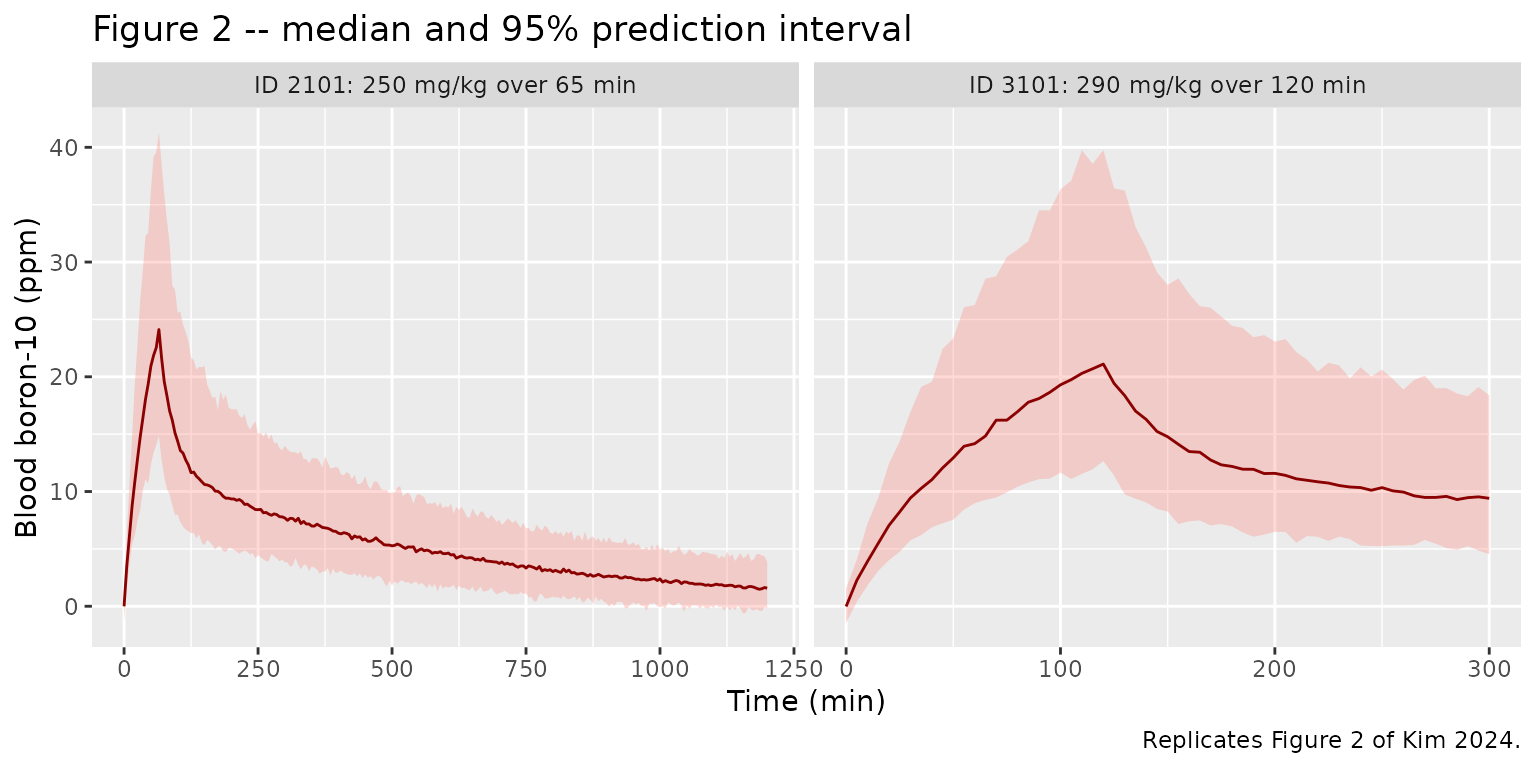
The published medians peak at about 24 ppm at the end of the 65-min infusion (patient 2101) and about 22 ppm at the end of the 120-min infusion (patient 3101); the published 95% interval at the 2101 peak spans roughly 14-41 ppm. The typical-value solve below checks the peaks deterministically.
ev_typ_fig2 <- events_fig2 |>
  dplyr::filter(id %in% c(1L, n_per_arm + 1L))
typ_fig2 <- rxode2::rxSolve(mod_typical, events = ev_typ_fig2, keep = "regimen") |>
  as.data.frame()
#> ℹ omega/sigma items treated as zero: 'etalkel', 'etalk12', 'etalk21', 'etalvc'
#> Warning: multi-subject simulation without without 'omega'

peak_fig2 <- tibble::tribble(
  ~regimen, ~time, ~figure2_median,
  "ID 2101: 250 mg/kg over 65 min", 65, 24.4,
  "ID 3101: 290 mg/kg over 120 min", 120, 22.0
) |>
  dplyr::left_join(
    dplyr::select(typ_fig2, regimen, time, Cc),
    by = c("regimen", "time")
  ) |>
  dplyr::mutate(pct_diff = 100 * (Cc - figure2_median) / figure2_median)

knitr::kable(
  peak_fig2 |>
    dplyr::rename(
      "Regimen" = regimen,
      "End of infusion (min)" = time,
      "Figure 2 median, digitised (ppm)" = figure2_median,
      "Packaged typical value (ppm)" = Cc,
      "Difference (%)" = pct_diff
    ),
  digits = 2,
  caption = "End-of-infusion typical-value concentration vs. the Figure 2 median."
)| Regimen | End of infusion (min) | Figure 2 median, digitised (ppm) | Packaged typical value (ppm) | Difference (%) |
|---|---|---|---|---|
| ID 2101: 250 mg/kg over 65 min | 65 | 24.4 | 24.78 | 1.56 |
| ID 3101: 290 mg/kg over 120 min | 120 | 22.0 | 21.98 | -0.07 |
Irradiation-window simulation (500 mg/kg over 180 min)
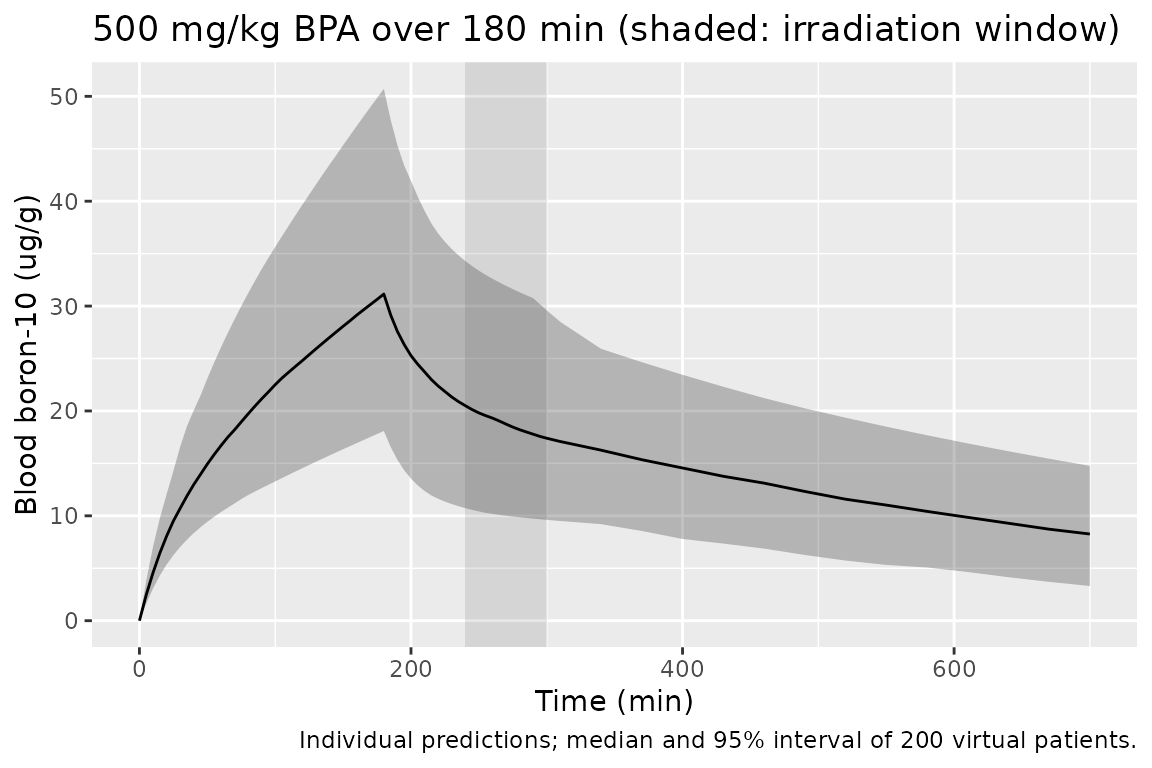
The paper’s sampling-schedule simulations use 500 mg/kg infused over 180 min, with neutron irradiation from 240 to 300 min. Section 3.3 states that the 95% interval of the mean blood boron level during irradiation was taken to be 10-30 ppm based on the population model.
rxode2::rxSetSeed(20240302)
n_sub <- 200L
obs_500 <- sort(unique(c(seq(0, 300, by = 5), seq(310, 2880, by = 30))))
events_500 <- dplyr::bind_rows(
  tibble::tibble(
    id = seq_len(n_sub), time = 0, amt = 500, rate = 500 / 180,
    evid = 1L, cmt = "central"
  ),
  tidyr::expand_grid(id = seq_len(n_sub), time = obs_500) |>
    dplyr::mutate(amt = NA_real_, rate = NA_real_, evid = 0L, cmt = "central")
) |>
  dplyr::mutate(treatment = "500 mg/kg over 180 min") |>
  dplyr::arrange(id, time, dplyr::desc(evid))

sim_500 <- rxode2::rxSolve(mod, events = events_500, keep = "treatment") |>
  as.data.frame()

# Mean concentration over the 240-300 min irradiation window, per subject
# (trapezoidal over the 5-min grid), using the individual prediction.
window_mean <- sim_500 |>
  dplyr::filter(time >= 240, time <= 300) |>
  dplyr::group_by(id) |>
  dplyr::summarise(
    cavg = sum(diff(time) * (head(Cc, -1) + tail(Cc, -1)) / 2) / 60,
    .groups = "drop"
  )

q_window <- quantile(window_mean$cavg, c(0.025, 0.5, 0.975))
knitr::kable(
  tibble::tibble(
    Statistic = c("2.5th percentile", "Median", "97.5th percentile"),
    "Mean blood boron-10, 240-300 min (ppm)" = unname(q_window)
  ),
  digits = 1,
  caption = "Simulated distribution of the irradiation-window mean (paper: 10-30 ppm)."
)| Statistic | Mean blood boron-10, 240-300 min (ppm) |
|---|---|
| 2.5th percentile | 10.1 |
| Median | 18.8 |
| 97.5th percentile | 32.0 |
# Centre and robust envelope only. On a 5000-subject cohort the model gives
# a median of 18.7 ppm (typical value 19.1), 10th percentile 12.6 and 90th
# percentile 27.5; each bound below is at least 4 standard errors of a
# 200-subject quantile away. The 2.5/97.5% tails are reported, not gated.
stopifnot(
  q_window[["50%"]] > 15, q_window[["50%"]] < 25,
  quantile(window_mean$cavg, 0.1) > 10,
  quantile(window_mean$cavg, 0.9) < 31
)
The simulated 95% interval of the irradiation-window mean (about 10-33 ppm) agrees with the 10-30 ppm interval the paper states for its population model.
sim_500 |>
  dplyr::filter(time <= 720) |>
  dplyr::group_by(time) |>
  dplyr::summarise(
    lo = quantile(Cc, 0.025), med = median(Cc), hi = quantile(Cc, 0.975),
    .groups = "drop"
  ) |>
  ggplot(aes(time, med)) +
  annotate("rect", xmin = 240, xmax = 300, ymin = -Inf, ymax = Inf, alpha = 0.15) +
  geom_ribbon(aes(ymin = lo, ymax = hi), alpha = 0.3) +
  geom_line() +
  labs(
    x = "Time (min)",
    y = "Blood boron-10 (ug/g)",
    title = "500 mg/kg BPA over 180 min (shaded: irradiation window)",
    caption = "Individual predictions; median and 95% interval of 200 virtual patients."
  )
PKNCA validation
The paper reports no NCA, so PKNCA is used to summarise the simulated
500 mg/kg cohort and, on a typical-value solve, to check AUC and
terminal half-life against the closed-form two-compartment values
(AUCinf = F * Dose / (kel * V1) with
F = 10/208.21 the boron-10 fraction, and
t1/2 = log(2) / beta).
nca_conc <- sim_500 |>
  dplyr::filter(!is.na(Cc)) |>
  dplyr::select(id, time, Cc, treatment)
nca_conc <- dplyr::bind_rows(
  nca_conc,
  nca_conc |> dplyr::distinct(id, treatment) |> dplyr::mutate(time = 0, Cc = 0)
) |>
  dplyr::distinct(id, treatment, time, .keep_all = TRUE) |>
  dplyr::arrange(id, treatment, time)

nca_dose <- events_500 |>
  dplyr::filter(evid == 1) |>
  dplyr::select(id, time, amt, treatment)

intervals <- data.frame(
  start = 0, end = Inf,
  cmax = TRUE, tmax = TRUE, aucinf.obs = TRUE, half.life = TRUE
)

nca_res <- PKNCA::pk.nca(PKNCA::PKNCAdata(
  PKNCA::PKNCAconc(nca_conc, Cc ~ time | treatment + id),
  PKNCA::PKNCAdose(nca_dose, amt ~ time | treatment + id),
  intervals = intervals
))
knitr::kable(
  summary(nca_res),
  caption = "PKNCA summary, 500 mg/kg BPA over 180 min (Cc in ug/g, time in min)."
)| start | end | treatment | N | cmax | tmax | half.life | aucinf.obs |
|---|---|---|---|---|---|---|---|
| 0 | Inf | 500 mg/kg over 180 min | 200 | 31.8 [27.2] | 180 [180, 180] | 386 [115] | 15800 [31.7] |
typ_500 <- rxode2::rxSolve(
  mod_typical,
  events = dplyr::filter(events_500, id == 1L),
  keep = "treatment"
) |>
  as.data.frame()
#> ℹ omega/sigma items treated as zero: 'etalkel', 'etalk12', 'etalk21', 'etalvc'
if (is.null(typ_500$id)) typ_500$id <- 1L

nca_typ <- PKNCA::pk.nca(PKNCA::PKNCAdata(
  PKNCA::PKNCAconc(
    dplyr::select(typ_500, id, time, Cc, treatment),
    Cc ~ time | treatment + id
  ),
  PKNCA::PKNCAdose(
    dplyr::filter(nca_dose, id == 1L),
    amt ~ time | treatment + id
  ),
  intervals = intervals
)) |>
  as.data.frame()

th <- exp(ui$theta)
kel <- th[["lkel"]]
k12 <- th[["lk12"]]
k21 <- th[["lk21"]]
v1 <- th[["lvc"]]
ksum <- kel + k12 + k21
beta <- (ksum - sqrt(ksum^2 - 4 * kel * k21)) / 2
closed <- c(
  aucinf.obs = 500 * (10 / 208.21) / (kel * v1),
  half.life = log(2) / beta
)

cmp_typ <- tibble::tibble(
  parameter = names(closed),
  closed_form = unname(closed),
  pknca = vapply(
    names(closed),
    function(p) nca_typ$PPORRES[nca_typ$PPTESTCD == p],
    numeric(1)
  )
) |>
  dplyr::mutate(pct_diff = 100 * (pknca - closed_form) / closed_form)

knitr::kable(
  cmp_typ |>
    dplyr::rename(
      "NCA parameter" = parameter,
      "Closed form" = closed_form,
      "PKNCA (typical value)" = pknca,
      "Difference (%)" = pct_diff
    ),
  digits = 2,
  caption = "Typical-value PKNCA vs. closed-form AUCinf (ug*min/g) and terminal half-life (min)."
)| NCA parameter | Closed form | PKNCA (typical value) | Difference (%) |
|---|---|---|---|
| aucinf.obs | 15882.42 | 15881.89 | 0.00 |
| half.life | 377.01 | 375.26 | -0.46 |
Assumptions and deviations
- V1 is per kilogram. Table 2 prints the unit of V1 as “L”, but the dose is given in mg/kg and Figure 4A prints an individual V1 of “0.22902 l/kg”. Only a per-kilogram volume reproduces the 20-35 ppm blood levels of Figures 2 and 4A (the deterministic Figure 4A check above), so the model is coded per kilogram: dose in mg/kg of BPA, V1 in L/kg.
-
Boron-10 conversion and units. The model state
holds BPA (mg/kg); the output is boron-10,
Cc = central * (10/208.21) / vc, using the paper’s factor (Methods 2.1). mg/L is reported as ug/g (ppm), which assumes a blood density of 1 g/mL, as the paper does. -
Residual-error scale. Table 2 prints the additive
and proportional residual terms (0.540 and 0.001) without saying whether
they are variances or standard deviations. The maintainers read them as
NONMEM
$SIGMAvariances, the same raw-estimate scale as the IIV rows of the same table (whose CV% values are exactlysqrt(exp(omega^2) - 1)), soaddSd = sqrt(0.540) = 0.73 ug/gandpropSd = sqrt(0.001) = 3.2%. Under the alternative SD reading (0.54 ug/g and 0.1%) the 95% prediction interval of Figure 2 moves visibly only in the low-concentration tail (by about 0.3 ppm at 1200 min for patient 2101), because the between-subject variability dominates; the figure cannot distinguish the two readings. - No covariates and no covariance. The source data were digitised from published figures, so no patient characteristics were available; Table 2 reports a diagonal IIV matrix.
- Figure 2 medians digitised. The end-of-infusion medians used in the Figure 2 check (24.4 and 22.0 ppm) were read from Figure 2 by the maintainers (about +/-0.5 ppm reading precision).
- No published NCA. The paper reports no NCA parameters, so there is no simulated-vs-published NCA table; PKNCA is checked against closed-form values instead.
- Europe PMC links no erratum or correction notice to this article as of 2026-10-29.