Nedosiran (Zhang 2025) • nlmixr2lib

Model and source

This paper contributes two model files:

Zhang_2025_nedosiran – the updated population PK model (Table 2).
Zhang_2025_nedosiran_uoxcr – the population PK/PD model in which that PK layer drives an effect compartment that inhibits spot urine oxalate-to-creatinine ratio (Uox/Cr) production (Table 3).

mod_pk <- readModelDb("Zhang_2025_nedosiran")
mod_pd <- readModelDb("Zhang_2025_nedosiran_uoxcr")

Citation: Zhang S, Gamallo P, Rawson V. Population Pharmacokinetic and Pharmacodynamic Modelling and Simulation for Nedosiran Clinical Development and Dose Guidance in Pediatric Patients with Primary Hyperoxaluria Type 1. Clin Pharmacokinet. 2025;64(8):1213-1227. doi:10.1007/s40262-025-01540-1
Article: https://doi.org/10.1007/s40262-025-01540-1
Supplement 1 (Tables S1-S4, demographics and eGFR formulas): https://doi.org/10.1007/s40262-025-01540-1
Supplement 2 (Figures S1-S2, GOF and VPC): https://doi.org/10.1007/s40262-025-01540-1

Nedosiran (Rivfloza) is a GalNAc-conjugated small interfering RNA that silences hepatic lactate dehydrogenase mRNA, reducing oxalate production in primary hyperoxaluria type 1 (PH1). The analysis supports a 3.5 mg/kg once-monthly (Q1M) regimen in children aged 2 to under 12 years.

Population

The PK model was fit to 2087 plasma concentrations from 148 participants across six trials (PHYOX1, PHYOX2, PHYOX3, PHYOX5, PHYOX6, PHYOX8): 85 healthy volunteers (57.4%), 49 patients with PH1 (33.1%) and 14 with PH2 (9.5%). The cohort was 35.8% female, 56.1% White / 19.6% Asian / 11.5% Black or African American / 6.1% Multiple / 4.7% Other / 2.0% Unknown, spanning 1.9-73 years of age, 11.1-129.5 kg body weight and 3.8-197 mL/min/1.73 m^2 eGFR (Supplementary Table S1). Renal function was normal in 41.9%, mildly impaired in 35.1%, moderately impaired in 6.8%, severely impaired in 4.7% and end-stage in 11.5%.

The PK/PD model was fit to 668 spot Uox/Cr observations from 41 patients with PH1 from PHYOX2, PHYOX3 and PHYOX8: 46.3% female, ages 2-46 years, body weight 11.9-115.9 kg, eGFR 35-197 mL/min/1.73 m^2 (Supplementary Table S2).

str(mod_pd()$population, max.level = 1)
#> List of 13
#>  $ species       : chr "human"
#>  $ n_subjects    : num 41
#>  $ n_studies     : num 3
#>  $ n_observations: num 668
#>  $ age_range     : chr "2-46 years"
#>  $ weight_range  : chr "11.9-115.9 kg"
#>  $ sex_female_pct: num 46.3
#>  $ race_ethnicity: Named num [1:5] 41.5 22 19.5 14.6 2.4
#>   ..- attr(*, "names")= chr [1:5] "White" "Multiple" "Asian" "Unknown" ...
#>  $ disease_state : chr "primary hyperoxaluria type 1"
#>  $ renal_function: chr "normal 36.6%, mild impairment 41.5%, moderate impairment 22.0%; eGFR 35-197 mL/min/1.73 m^2"
#>  $ dose_range    : chr "136 or 170 mg SC once-monthly (age >= 12 years) and 3.5 mg/kg SC once-monthly capped at 136 or 170 mg (age < 12 years)"
#>  $ regions       : chr "multinational"
#>  $ notes         : chr "Patients with primary hyperoxaluria type 1 and at least one post-baseline spot Uox/Cr value from PHYOX2 (NCT038"| __truncated__

Source trace

Every ini() entry carries an in-file comment naming its source location. The tables below collect them.

PK model (Table 2)

Parameter	Value	Source
`lcl` (CL/F)	6.10 L/h	Table 2
`lvc` (Vc/F)	148 L	Table 2
`lq` (Q/F)	2.79 L/h	Table 2
`lvp` (Vp/F)	6560 L	Table 2
`lvmax` (Vmax)	3.37 mg/h	Table 2
`lkm` (KM)	248 ng/mL	Table 2
`lka1` (slow pathway)	0.212 1/h	Table 2
`lka2` (fast pathway)	14.9 1/h	Table 2
`logitffo` (FR1)	0.692 -> qlogis = 0.8095	Table 2
`e_wt_cl_q`	0.750 (fixed)	Table 2, CL.BW
`e_wt_vc_vp`	1.00 (fixed)	Table 2, V.BW
`e_wt_ka`	-0.221	Table 2, ka.BW
`e_wt_vmax`	0.492	Table 2, Vmax.BW
`e_crcl_cl`	0.969	Table 2, CL.EGFR
`e_crcl_vc`	0.174	Table 2, Vc.EGFR
`e_ph1_ka1`	1.32	Table 2, Ka1.PH
IIV `etalvc`	27.9 CV% -> 0.07496	Table 2
IIV `etalka1`	49.3 CV% -> 0.21757	Table 2
IIV `etalka2`	53.4 CV% -> 0.25088	Table 2
IIV `etalvmax`	35.1 CV% -> 0.11618	Table 2
IIV `etalogitffo`	0.342 SD (logit) -> 0.11696	Table 2
`expSd`	30.8 CV% -> 0.30105	Table 2, ExpError
Covariate equations	see below	Table 2 footnote
ODE structure	dual transit + 2-cmt + MM	Fig. 1

The Table 2 footnote prints the covariate model as

CL/F = TVCL  x (BW/BWref)^CL.BW x (eGFR/eGFRref)^CL.eGFR
Vc/F = TVVc  x (BW/BWref)^V.BW  x (eGFR/eGFRref)^Vc.eGFR
Q/F  = TVQ   x (BW/BWref)^CL.BW
Vp/F = TVVp  x (BW/BWref)^V.BW
Ka1  = TVKa1 x (BW/BWref)^ka.BW x (Ka1.PH)^PH
Ka2  = TVKa2 x (BW/BWref)^ka.BW
Vmax = TVVmax x (BW/BWref)

with BWref = 70 kg, eGFRref = 90 mL/min/1.73 m^2 and PH = 1 for PH1.

PK/PD model (Table 3)

Parameter	Value	Source
`lrbase` (BSL)	264 mmol/mol	Table 3
`limax` (Imax)	0.687	Table 3
`lic50` (IC50)	1.68 ng/mL	Table 3
`lhill` (gamma)	2.56 (fixed)	Table 3
`lkout` (kout)	0.338 1/wk (fixed) -> /168 for 1/h	Table 3
`lke0` (ke0)	ln(2)/lambda, lambda = 21.9 wk (fixed)	Table 3 + Fig. 1
`e_age_rbase`	-0.450	Table 3, AGE.BSL
IIV `etalrbase`	42.2 CV% -> 0.16389	Table 3
IIV `etalic50`	85.2 CV% -> 0.54575	Table 3
`propSd_uoxcr`	35.5 CV% -> 0.355	Table 3, PropError
Turnover + effect cmt	`kin(1-Eff) - koutuoxcr`	Fig. 1

The Table 3 footnote gives BSL = TVBSL x (AGE/AGEref)^AGE.BSL with AGEref = 6 years.

Virtual cohort

Individual patient data are not public. The cohorts below approximate the published trial demographics (Supplementary Tables S1, S2 and S4) and the virtual population described in Sect. 2.2.1 (WHO weight-for-age for children, NHANES for adults, uniform sampling across sex, renal categories defined by eGFR bands).

TAU   <- 672L    # once-monthly dosing interval, hours (28 days)
NDOSE <- 7L      # 7 monthly doses spans the 26-week evaluation window

# Renal categories exactly as defined in Sect. 2.2.1 / Fig. 5.
egfr_band <- function(category, n) {
  switch(
    category,
    normal   = runif(n,  90, 130),
    mild     = runif(n,  60,  89),
    moderate = runif(n,  30,  59)
  )
}

# Build one arm: `n` subjects, monthly SC dosing, observations on a named ODE
# state. Each SC injection is entered as TWO simultaneous dose records both
# carrying the full injected amount; the model's f(depot) / f(depot2) apply the
# FR1 / (1 - FR1) split.
make_arm <- function(n, wt, age, egfr, dose, obs_times, obs_cmt,
                     arm, id_offset = 0L) {
  ids <- id_offset + seq_len(n)
  covs <- tibble(id = ids, WT = wt, AGE = age, CRCL = egfr,
                 DIS_PH1 = 1, arm = arm)

  dosing <- tibble(
    id   = rep(ids, each = 2L),
    time = 0,
    amt  = rep(dose, each = 2L),
    evid = 1L,
    cmt  = rep(c("depot", "depot2"), times = n),
    ii   = TAU,
    addl = NDOSE - 1L
  )
  obs <- tidyr::crossing(id = ids, time = obs_times) |>
    mutate(amt = NA_real_, evid = 0L, cmt = obs_cmt, ii = 0, addl = 0L)

  bind_rows(dosing, obs) |>
    left_join(covs, by = "id") |>
    arrange(id, time, desc(evid))
}

PK simulation

set.seed(20250818)
N_ARM <- 150L

# Body weights: WHO-style medians for the paediatric age bands and an adult
# distribution consistent with Supplementary Table S1.
wt_for <- function(age_lo, age_hi, n) {
  med <- c("2" = 15, "6" = 24, "9" = 35, "12" = 55, "18" = 75)[
    as.character(age_lo)]
  rlnorm(n, log(med), 0.22)
}

pk_bands <- tibble::tribble(
  ~arm,               ~age_lo, ~age_hi,
  "2 to <6 y",         2,       6,
  "6 to <9 y",         6,       9,
  "9 to <12 y",        9,      12,
  "12 to <18 y",      12,      18,
  ">=18 y",           18,      55
)

# The first and seventh dosing intervals are sampled on the SAME dense grid so
# that the accumulation ratio compares like with like; a coarse first-cycle
# grid would miss the ~7 h peak and inflate the ratio.
dense_grid <- c(seq(0, 24, by = 0.5), seq(26, 72, by = 4), seq(96, TAU, by = 24))
pk_obs_times <- sort(unique(c(
  dense_grid,
  seq(0, 6 * TAU, by = 24),
  6 * TAU + dense_grid
)))

pk_events <- do.call(bind_rows, lapply(seq_len(nrow(pk_bands)), function(i) {
  b <- pk_bands[i, ]
  wt  <- wt_for(b$age_lo, b$age_hi, N_ARM)
  age <- runif(N_ARM, b$age_lo, b$age_hi)
  # Weight-band dosing rule from the trials: 3.5 mg/kg (cap 170 mg) under
  # 12 years; 170 mg at >=50 kg and 136 mg at <50 kg from 12 years.
  dose <- if (b$age_lo < 12) pmin(170, 3.5 * wt) else ifelse(wt >= 50, 170, 136)
  make_arm(N_ARM, wt, age, egfr_band("normal", N_ARM), dose,
           pk_obs_times, "central", b$arm, id_offset = (i - 1L) * N_ARM)
}))

stopifnot(!anyDuplicated(pk_events[pk_events$evid == 0, c("id", "time")]))

sim_pk <- rxode2::rxSolve(mod_pk, events = pk_events,
                          keep = c("arm", "WT", "CRCL"),
                          addDosing = FALSE) |>
  as.data.frame()
#> ℹ parameter labels from comments will be replaced by 'label()'
stopifnot(length(unique(sim_pk$id)) == N_ARM * nrow(pk_bands))

sim_pk |>
  filter(time >= 6 * TAU) |>
  mutate(tad = time - 6 * TAU,
         arm = factor(arm, levels = pk_bands$arm)) |>
  group_by(arm, tad) |>
  summarise(Q05 = quantile(Cc, 0.05), Q50 = median(Cc),
            Q95 = quantile(Cc, 0.95), .groups = "drop") |>
  ggplot(aes(tad, Q50)) +
  geom_ribbon(aes(ymin = Q05, ymax = Q95), alpha = 0.25, fill = "steelblue") +
  geom_line(colour = "steelblue4") +
  geom_hline(yintercept = 1, linetype = "dotted") +
  facet_wrap(~arm) +
  scale_x_continuous(limits = c(0, 168)) +
  scale_y_log10() +
  labs(x = "Time after the 7th monthly dose (h)", y = "Nedosiran (ng/mL)",
       caption = paste("Dotted line = 1.0 ng/mL assay LLOQ.",
                       "Compare Supplementary Fig. S2 of Zhang 2025."))
#> Warning: Removed 105 rows containing missing values or values outside the scale range
#> (`geom_ribbon()`).
#> Warning: Removed 105 rows containing missing values or values outside the scale range
#> (`geom_line()`).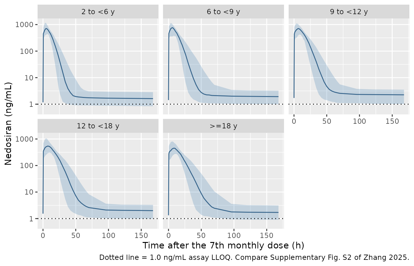

Simulated steady-state nedosiran concentration-time profiles by age band.

PKNCA validation

Concentrations below the 1.0 ng/mL assay LLOQ are excluded, as they were from the published analysis. Two intervals are computed: exposure metrics (Cmax,ss, Tmax, AUCtau,ss, Cav) over the full monthly interval, and the half-life over a 0-48 h window, because the published 4.6-13.8 h range describes the disposition phase the trials actually sampled (see Assumptions and deviations).

LLOQ <- 1.0   # ng/mL, Sect. 2.1.1

nca_conc <- sim_pk |>
  filter(time >= 6 * TAU, !is.na(Cc)) |>
  mutate(tad = time - 6 * TAU) |>
  # Sect. 2.1.2: "Samples with a LLOQ value below 1.0 ng/mL were excluded from
  # the PK analysis." Retaining them lets lambda.z reach into the very slow
  # peripheral phase (Vp/F 6560 L), which the trials never sampled. The
  # pre-dose record is kept so PKNCA can anchor the interval at time zero.
  filter(Cc >= LLOQ | tad == 0) |>
  select(id, tad, Cc, arm) |>
  distinct(id, arm, tad, .keep_all = TRUE) |>
  arrange(id, arm, tad)

conc_obj <- PKNCA::PKNCAconc(as.data.frame(nca_conc), Cc ~ tad | arm + id)

nca_dose <- pk_events |>
  filter(evid == 1, cmt == "depot") |>
  distinct(id, arm, amt) |>
  mutate(tad = 0)
dose_obj <- PKNCA::PKNCAdose(as.data.frame(nca_dose), amt ~ tad | arm + id)

intervals <- data.frame(
  start     = c(0, 0),
  end       = c(TAU, 48),
  cmax      = c(TRUE,  FALSE),
  tmax      = c(TRUE,  FALSE),
  auclast   = c(TRUE,  FALSE),
  cav       = c(TRUE,  FALSE),
  half.life = c(FALSE, TRUE)
)

nca_res <- suppressWarnings(
  PKNCA::pk.nca(PKNCA::PKNCAdata(conc_obj, dose_obj, intervals = intervals))
)

as.data.frame(nca_res$result) |>
  filter(PPTESTCD %in% c("cmax", "tmax", "auclast", "cav", "half.life")) |>
  group_by(arm, PPTESTCD) |>
  summarise(median = median(PPORRES, na.rm = TRUE), .groups = "drop") |>
  pivot_wider(names_from = PPTESTCD, values_from = median) |>
  mutate(across(where(is.numeric), ~ signif(.x, 3))) |>
  rename("Age band" = arm, "AUCtau,ss (ng*h/mL)" = auclast,
         "Cav,ss (ng/mL)" = cav, "Cmax,ss (ng/mL)" = cmax,
         "t1/2 0-48 h (h)" = half.life, "Tmax (h)" = tmax) |>
  knitr::kable(caption = "Median simulated steady-state NCA by age band.")

Median simulated steady-state NCA by age band.
Age band	AUCtau,ss (ng*h/mL)	Cav,ss (ng/mL)	Cmax,ss (ng/mL)	t1/2 0-48 h (h)	Tmax (h)
12 to <18 y	12700	18.9	555	5.43	7.5
2 to <6 y	10900	16.3	726	3.96	5.0
6 to <9 y	12900	19.1	779	4.22	5.5
9 to <12 y	14300	21.2	735	4.74	6.5
>=18 y	10800	16.1	452	5.91	7.5

Comparison against published NCA

The paper reports Tmax qualitatively (“peaked approximately 6-12 h post-dose”, Sect. 4) and cites a plasma half-life of 4.6-13.8 h from the PHYOX1 analysis. Both references below are the midpoints of those published ranges.

published <- tibble::tribble(
  ~arm,          ~tmax, ~half.life,
  ">=18 y",       9.0,   9.2
)

cmp <- nlmixr2lib::ncaComparisonTable(
  simulated     = nca_res,
  reference     = published,
  by            = "arm",
  params        = c("tmax", "half.life"),
  units         = c(tmax = "h", half.life = "h"),
  tolerance_pct = 20
)
knitr::kable(cmp, caption = paste(
  "Simulated vs published nedosiran NCA in adults.",
  "* differs from the published midpoint by >20%."))

Simulated vs published nedosiran NCA in adults. * differs from the published midpoint by >20%.
NCA parameter	arm	Reference	Simulated	% diff
Tmax (h)	>=18 y	9	7.5	-16.7%
t½ (h)	>=18 y	9.2	5.91	-35.7%*

The half-life row is starred because it differs from the 9.2 h midpoint by more than 20%. Both simulated values nonetheless fall inside the published ranges – Tmax within 6-12 h and half-life within 4.6-13.8 h – which is what the paper actually reports; the midpoints are an artefact of needing a single reference number for the comparison. The assertions below test membership of the published ranges rather than proximity to their midpoints.

adult <- as.data.frame(nca_res$result) |> filter(arm == ">=18 y")
med <- function(p) median(adult$PPORRES[adult$PPTESTCD == p], na.rm = TRUE)

# Sect. 4: concentrations peaked approximately 6-12 h post-dose.
stopifnot(med("tmax") >= 6, med("tmax") <= 12)
# Sect. 4 / ref 18: plasma half-life 4.6-13.8 h.
stopifnot(med("half.life") >= 4.6, med("half.life") <= 13.8)

# Sect. 4: "No accumulation of nedosiran at steady state, with plasma
# concentrations close to or below LLOQ before each monthly dose."
acc <- sim_pk |>
  filter(arm == ">=18 y") |>
  mutate(cycle = ifelse(time <= TAU, "first", ifelse(time > 6 * TAU, "seventh", NA))) |>
  filter(!is.na(cycle)) |>
  group_by(id, cycle) |>
  summarise(cmax = max(Cc), .groups = "drop") |>
  pivot_wider(names_from = cycle, values_from = cmax) |>
  summarise(accumulation_ratio = median(seventh / first))

trough <- sim_pk |>
  filter(arm == ">=18 y", abs(time - 7 * TAU) < 1e-6) |>
  summarise(median_trough = median(Cc))

tibble(Quantity = c("Cmax accumulation ratio (dose 7 / dose 1)",
                    "Median pre-dose concentration (ng/mL)"),
       Value = signif(c(acc$accumulation_ratio, trough$median_trough), 3),
       Published = c("no accumulation (ratio ~1)",
                     "close to or below 1.0 ng/mL LLOQ")) |>
  knitr::kable(caption = "Steady-state accumulation checks (Zhang 2025 Sect. 4).")

Steady-state accumulation checks (Zhang 2025 Sect. 4).
Quantity	Value	Published
Cmax accumulation ratio (dose 7 / dose 1)	1.00	no accumulation (ratio ~1)
Median pre-dose concentration (ng/mL)	1.42	close to or below 1.0 ng/mL LLOQ


stopifnot(abs(acc$accumulation_ratio - 1) < 0.10)

Covariate effects on exposure (Figure 4)

Figure 4 reports fold changes in AUCtau,ss and Cmax,ss relative to a reference PH1 adult of 75 kg with eGFR 100 mL/min/1.73 m^2 on 170 mg Q1M. These are typical-value comparisons, so the random effects are zeroed.

mod_pk_typ <- rxode2::zeroRe(mod_pk)
#> ℹ parameter labels from comments will be replaced by 'label()'

exposure_at <- function(wt, egfr, ph1, dose = 170) {
  ev <- make_arm(1L, wt, 30, egfr, dose,
                 obs_times = 6 * TAU + seq(0, TAU, by = 0.25),
                 obs_cmt = "central", arm = "x")
  ev$DIS_PH1 <- ph1
  s <- as.data.frame(rxode2::rxSolve(mod_pk_typ, events = ev,
                                     addDosing = FALSE))
  s <- s[s$time >= 6 * TAU, ]
  c(auc  = sum(diff(s$time) * (head(s$Cc, -1) + tail(s$Cc, -1)) / 2),
    cmax = max(s$Cc))
}

ref <- exposure_at(75, 100, 1)
#> ℹ omega/sigma items treated as zero: 'etalvc', 'etalka1', 'etalka2', 'etalvmax', 'etalogitffo'

scenarios <- tibble::tribble(
  ~label,                                   ~wt, ~egfr, ~ph1, ~pub_auc, ~pub_cmax,
  "Moderate renal impairment (eGFR 45)",     75,    45,    1,     1.42,      1.27,
  "PH2 / healthy volunteer (PH1 = 0)",       75,   100,    0,       NA,        NA,
  "Body weight 95th percentile (100 kg)",   100,   100,    1,     0.76,      0.71,
  "Body weight 5th percentile (48 kg)",      48,   100,    1,     1.45,      1.57
)

exp_mat <- vapply(
  seq_len(nrow(scenarios)),
  function(i) exposure_at(scenarios$wt[i], scenarios$egfr[i], scenarios$ph1[i]),
  numeric(2)
)
#> ℹ omega/sigma items treated as zero: 'etalvc', 'etalka1', 'etalka2', 'etalvmax', 'etalogitffo'
#> ℹ omega/sigma items treated as zero: 'etalvc', 'etalka1', 'etalka2', 'etalvmax', 'etalogitffo'
#> ℹ omega/sigma items treated as zero: 'etalvc', 'etalka1', 'etalka2', 'etalvmax', 'etalogitffo'
#> ℹ omega/sigma items treated as zero: 'etalvc', 'etalka1', 'etalka2', 'etalvmax', 'etalogitffo'

fold <- scenarios |>
  mutate(`AUCtau,ss fold` = signif(exp_mat["auc", ] / ref[["auc"]], 3),
         `Cmax,ss fold`   = signif(exp_mat["cmax", ] / ref[["cmax"]], 3)) |>
  select(label, `AUCtau,ss fold`, pub_auc, `Cmax,ss fold`, pub_cmax) |>
  rename("Scenario" = label, "Published AUC fold" = pub_auc,
         "Published Cmax fold" = pub_cmax)

knitr::kable(fold, caption = paste(
  "Replicates Figure 4 / Sect. 3.2 of Zhang 2025.",
  "Reference: PH1 adult, 75 kg, eGFR 100, 170 mg Q1M."))

Replicates Figure 4 / Sect. 3.2 of Zhang 2025. Reference: PH1 adult, 75 kg, eGFR 100, 170 mg Q1M.
Scenario	AUCtau,ss fold	Published AUC fold	Cmax,ss fold	Published Cmax fold
Moderate renal impairment (eGFR 45)	1.420	1.42	1.260	1.27
PH2 / healthy volunteer (PH1 = 0)	0.977	NA	0.858	NA
Body weight 95th percentile (100 kg)	0.784	0.76	0.740	0.71
Body weight 5th percentile (48 kg)	1.470	1.45	1.600	1.57

The moderate-renal-impairment row is a direct numerical match to the published values (1.42 and 1.27) using the midpoint of the 30-59 mL/min/1.73 m^2 band. The PH subtype row lies inside the [0.80, 1.25] bioequivalence limits drawn on Figure 4, consistent with the paper’s statement that “the PH subtype status showed no effect on exposure of nedosiran.”

mod_row <- fold[1, ]
stopifnot(abs(mod_row$`AUCtau,ss fold` - 1.42) < 0.10)
stopifnot(abs(mod_row$`Cmax,ss fold` - 1.27) < 0.10)
ph_row <- fold[2, ]
stopifnot(ph_row$`AUCtau,ss fold` > 0.80, ph_row$`AUCtau,ss fold` < 1.25)

The body-weight rows depend on the 5th and 95th weight percentiles of the participants aged >=12 years, which the paper does not report. Weights of 48 kg and 100 kg reproduce the published fold changes closely and are plausible percentiles for that cohort (Supplementary Table S1 gives an overall weight range of 11.1-129.5 kg). The curve below shows the full relationship.

wt_grid <- seq(35, 120, by = 5)
wt_curve <- do.call(rbind, lapply(wt_grid, function(w) {
  e <- exposure_at(w, 100, 1)
  data.frame(WT = w, AUC = e["auc"] / ref["auc"], Cmax = e["cmax"] / ref["cmax"])
}))
#> ℹ omega/sigma items treated as zero: 'etalvc', 'etalka1', 'etalka2', 'etalvmax', 'etalogitffo'
#> ℹ omega/sigma items treated as zero: 'etalvc', 'etalka1', 'etalka2', 'etalvmax', 'etalogitffo'
#> ℹ omega/sigma items treated as zero: 'etalvc', 'etalka1', 'etalka2', 'etalvmax', 'etalogitffo'
#> ℹ omega/sigma items treated as zero: 'etalvc', 'etalka1', 'etalka2', 'etalvmax', 'etalogitffo'
#> ℹ omega/sigma items treated as zero: 'etalvc', 'etalka1', 'etalka2', 'etalvmax', 'etalogitffo'
#> ℹ omega/sigma items treated as zero: 'etalvc', 'etalka1', 'etalka2', 'etalvmax', 'etalogitffo'
#> ℹ omega/sigma items treated as zero: 'etalvc', 'etalka1', 'etalka2', 'etalvmax', 'etalogitffo'
#> ℹ omega/sigma items treated as zero: 'etalvc', 'etalka1', 'etalka2', 'etalvmax', 'etalogitffo'
#> ℹ omega/sigma items treated as zero: 'etalvc', 'etalka1', 'etalka2', 'etalvmax', 'etalogitffo'
#> ℹ omega/sigma items treated as zero: 'etalvc', 'etalka1', 'etalka2', 'etalvmax', 'etalogitffo'
#> ℹ omega/sigma items treated as zero: 'etalvc', 'etalka1', 'etalka2', 'etalvmax', 'etalogitffo'
#> ℹ omega/sigma items treated as zero: 'etalvc', 'etalka1', 'etalka2', 'etalvmax', 'etalogitffo'
#> ℹ omega/sigma items treated as zero: 'etalvc', 'etalka1', 'etalka2', 'etalvmax', 'etalogitffo'
#> ℹ omega/sigma items treated as zero: 'etalvc', 'etalka1', 'etalka2', 'etalvmax', 'etalogitffo'
#> ℹ omega/sigma items treated as zero: 'etalvc', 'etalka1', 'etalka2', 'etalvmax', 'etalogitffo'
#> ℹ omega/sigma items treated as zero: 'etalvc', 'etalka1', 'etalka2', 'etalvmax', 'etalogitffo'
#> ℹ omega/sigma items treated as zero: 'etalvc', 'etalka1', 'etalka2', 'etalvmax', 'etalogitffo'
#> ℹ omega/sigma items treated as zero: 'etalvc', 'etalka1', 'etalka2', 'etalvmax', 'etalogitffo'

wt_curve |>
  pivot_longer(c(AUC, Cmax), names_to = "Metric", values_to = "Fold") |>
  ggplot(aes(WT, Fold, colour = Metric)) +
  geom_line(linewidth = 0.9) +
  geom_hline(yintercept = c(0.76, 1.45), linetype = "dashed", colour = "grey40") +
  geom_hline(yintercept = c(0.71, 1.57), linetype = "dotted", colour = "grey40") +
  labs(x = "Body weight (kg)", y = "Fold change vs 75 kg reference",
       caption = paste("Dashed = published AUC folds (0.76, 1.45);",
                       "dotted = published Cmax folds (0.71, 1.57)."))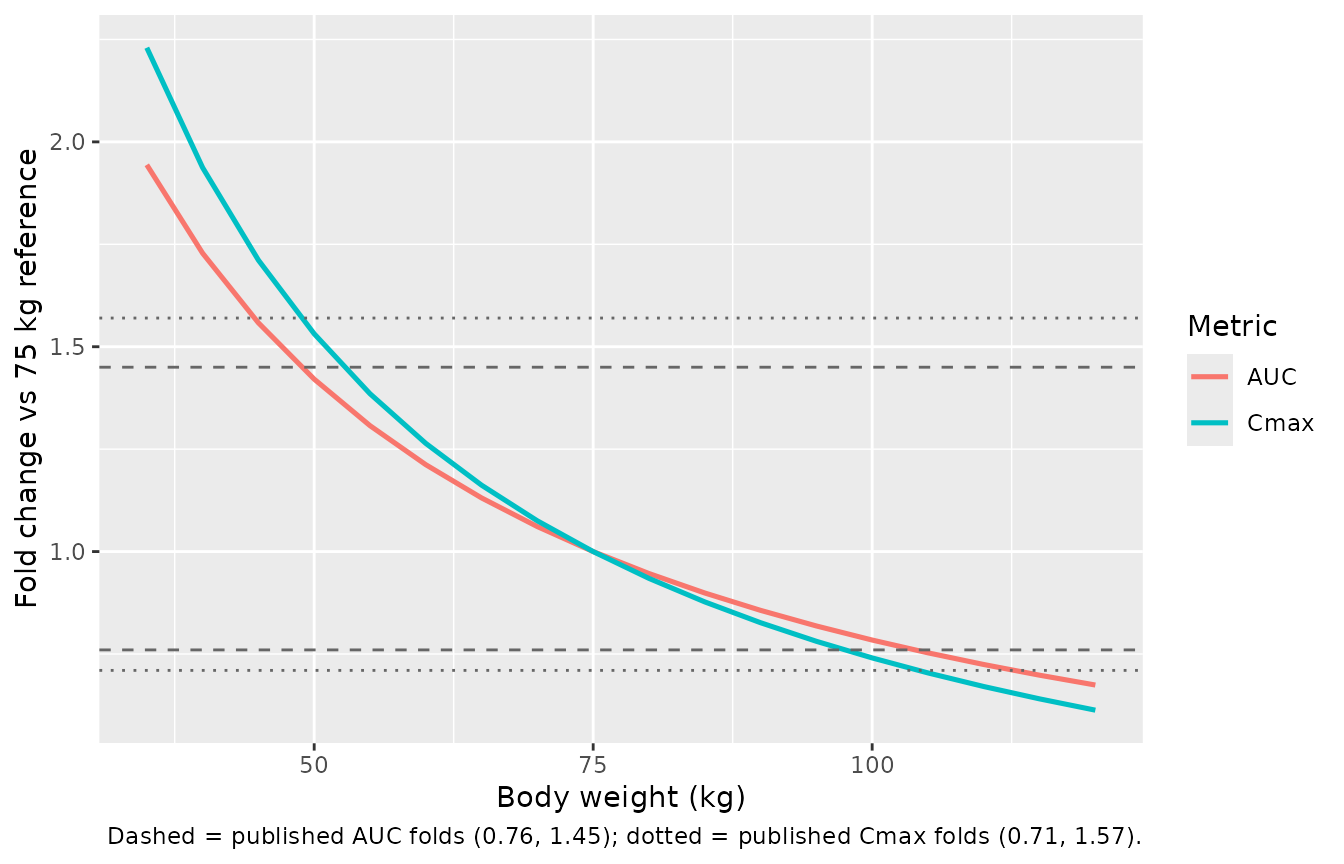

Exposure fold change vs body weight; horizontal lines are the published 5th/95th percentile values.

PK/PD: spot Uox/Cr response

Because kin = kout * rbase and uoxcr(0) = rbase, the relative Uox/Cr profile is independent of the baseline. Baseline IIV and the age effect on baseline therefore scale the absolute curve but not the percent reduction – the endpoint the paper reports.

set.seed(20250819)
N_PD <- 200L

pd_groups <- tibble::tribble(
  ~arm,                                       ~age_lo, ~age_hi, ~wt_med, ~rule,
  "170 mg, >=12 y, >=50 kg",                     18,      55,      75,   "adult",
  "3.5 mg/kg (cap 170), 2 to <6 y",               2,       6,      15,   "peds",
  "3.5 mg/kg (cap 170), 6 to <9 y",               6,       9,      24,   "peds",
  "3.5 mg/kg (cap 170), 9 to <12 y, <50 kg",      9,      12,      35,   "peds"
)

pd_obs_times <- seq(0, 26 * 168, by = 168)   # weekly, 26 weeks

build_pd <- function(g, category, id_offset) {
  wt <- rlnorm(N_PD, log(g$wt_med), 0.22)
  if (g$rule == "adult") wt <- pmax(50, wt) else if (g$age_lo == 9) wt <- pmin(50, wt)
  age  <- runif(N_PD, g$age_lo, g$age_hi)
  dose <- if (g$rule == "adult") rep(170, N_PD) else pmin(170, 3.5 * wt)
  make_arm(N_PD, wt, age, egfr_band(category, N_PD), dose,
           pd_obs_times, "uoxcr", g$arm, id_offset = id_offset) |>
    mutate(renal = category)
}

cats <- c("normal", "mild", "moderate")
grid <- tidyr::crossing(gi = seq_len(nrow(pd_groups)), category = cats)
pd_events <- do.call(bind_rows, lapply(seq_len(nrow(grid)), function(k) {
  build_pd(pd_groups[grid$gi[k], ], grid$category[k], (k - 1L) * N_PD)
}))

sim_pd <- rxode2::rxSolve(mod_pd, events = pd_events,
                          keep = c("arm", "renal", "WT", "AGE"),
                          addDosing = FALSE) |>
  as.data.frame()
#> ℹ parameter labels from comments will be replaced by 'label()'

pd_rel <- sim_pd |>
  group_by(id) |>
  mutate(pct_change = 100 * (uoxcr / uoxcr[which.min(time)] - 1),
         week = time / 168) |>
  ungroup()

pd_rel |>
  mutate(renal = factor(renal, levels = cats),
         arm   = factor(arm, levels = pd_groups$arm)) |>
  group_by(arm, renal, week) |>
  summarise(Q05 = quantile(pct_change, 0.05), Q50 = median(pct_change),
            Q95 = quantile(pct_change, 0.95), .groups = "drop") |>
  ggplot(aes(week, Q50, colour = arm, fill = arm)) +
  geom_line(linewidth = 0.8) +
  geom_line(aes(y = Q05), linetype = "dashed", linewidth = 0.3) +
  geom_line(aes(y = Q95), linetype = "dashed", linewidth = 0.3) +
  geom_hline(yintercept = -60, colour = "grey30", linetype = "dotted") +
  facet_wrap(~renal) +
  labs(x = "Week", y = "Change in spot Uox/Cr from baseline (%)",
       colour = NULL, fill = NULL,
       caption = "Dotted line = the 60% reduction threshold used in Table 4.") +
  theme(legend.position = "bottom") +
  guides(colour = guide_legend(nrow = 4))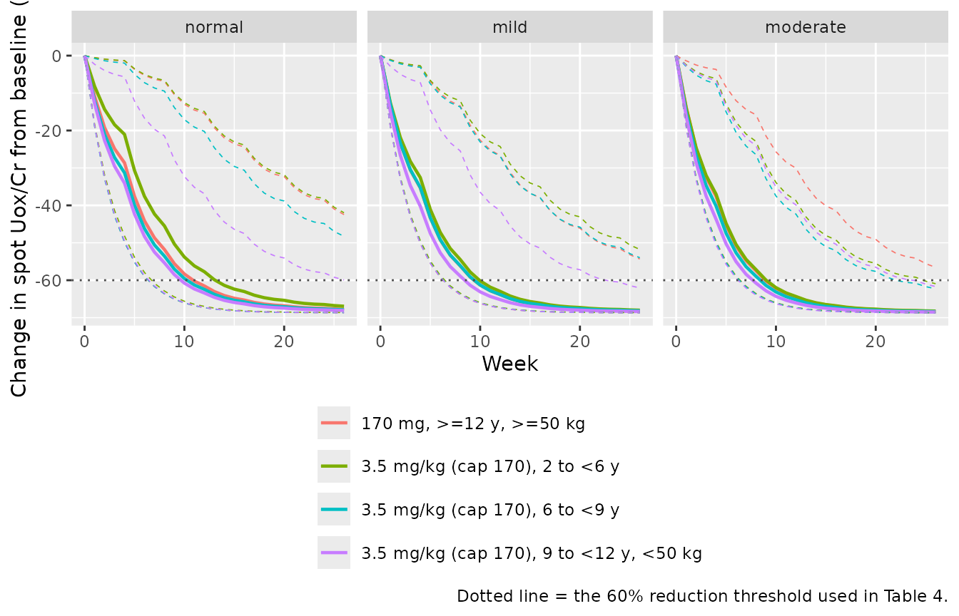

Replicates Figures 6-7 of Zhang 2025: simulated change in spot Uox/Cr from baseline.

# Sect. 3.2.2: "the predicted median time from start of treatment to reach the
# plateau was similar, at around 12 to 16 weeks."
plateau <- pd_rel |>
  group_by(arm, renal, week) |>
  summarise(med = median(pct_change), .groups = "drop") |>
  group_by(arm, renal) |>
  summarise(week_90pct = week[which(med <= 0.9 * min(med))[1]], .groups = "drop")

tibble(Quantity = "Median week reaching 90% of maximum effect",
       Range = paste0(min(plateau$week_90pct), " to ",
                      max(plateau$week_90pct), " weeks"),
       Published = "around 12 to 16 weeks") |>
  knitr::kable(caption = "Time to plateau (Zhang 2025 Sect. 3.2.2).")

Time to plateau (Zhang 2025 Sect. 3.2.2).
Quantity	Range	Published
Median week reaching 90% of maximum effect	9 to 14 weeks	around 12 to 16 weeks

Table 4: percentage reaching a 60% Uox/Cr reduction at week 26

published_t4 <- tibble::tribble(
  ~arm,                                        ~normal, ~mild, ~moderate,
  "170 mg, >=12 y, >=50 kg",                      78.1,  88.0,      91.1,
  "3.5 mg/kg (cap 170), 2 to <6 y",               82.0,  88.9,      90.7,
  "3.5 mg/kg (cap 170), 6 to <9 y",               88.3,  92.3,      94.8,
  "3.5 mg/kg (cap 170), 9 to <12 y, <50 kg",      89.4,  93.7,      96.9
) |>
  pivot_longer(-arm, names_to = "renal", values_to = "Published (%)")

simulated_t4 <- pd_rel |>
  filter(week == 26) |>
  group_by(arm, renal) |>
  summarise(`Simulated (%)` = round(100 * mean(pct_change <= -60), 1),
            .groups = "drop")

t4 <- left_join(simulated_t4, published_t4, by = c("arm", "renal")) |>
  mutate(Difference = round(`Simulated (%)` - `Published (%)`, 1),
         renal = factor(renal, levels = cats),
         arm = factor(arm, levels = pd_groups$arm)) |>
  arrange(arm, renal) |>
  rename("Group" = arm, "Renal function" = renal)

knitr::kable(t4, caption = paste(
  "Replicates Table 4 of Zhang 2025: percentage of PH1 patients reaching a",
  "60% spot Uox/Cr reduction after 26 weeks."))

Replicates Table 4 of Zhang 2025: percentage of PH1 patients reaching a 60% spot Uox/Cr reduction after 26 weeks.
Group	Renal function	Simulated (%)	Published (%)	Difference
170 mg, >=12 y, >=50 kg	normal	82.5	78.1	4.4
170 mg, >=12 y, >=50 kg	mild	92.0	88.0	4.0
170 mg, >=12 y, >=50 kg	moderate	92.5	91.1	1.4
3.5 mg/kg (cap 170), 2 to <6 y	normal	82.5	82.0	0.5
3.5 mg/kg (cap 170), 2 to <6 y	mild	89.0	88.9	0.1
3.5 mg/kg (cap 170), 2 to <6 y	moderate	95.5	90.7	4.8
3.5 mg/kg (cap 170), 6 to <9 y	normal	87.5	88.3	-0.8
3.5 mg/kg (cap 170), 6 to <9 y	mild	93.0	92.3	0.7
3.5 mg/kg (cap 170), 6 to <9 y	moderate	96.5	94.8	1.7
3.5 mg/kg (cap 170), 9 to <12 y, <50 kg	normal	94.5	89.4	5.1
3.5 mg/kg (cap 170), 9 to <12 y, <50 kg	mild	97.0	93.7	3.3
3.5 mg/kg (cap 170), 9 to <12 y, <50 kg	moderate	96.5	96.9	-0.4

# The paper's central claim: children on 3.5 mg/kg Q1M respond comparably to
# the >=12 y / >=50 kg reference group on 170 mg Q1M.
ref_norm <- t4$`Simulated (%)`[t4$Group == "170 mg, >=12 y, >=50 kg" &
                                 t4$`Renal function` == "normal"]
peds_norm <- t4$`Simulated (%)`[grepl("3.5 mg/kg", t4$Group) &
                                  t4$`Renal function` == "normal"]
stopifnot(all(peds_norm >= ref_norm - 10))

# Response increases as renal function declines (exposure rises).
by_arm <- split(t4, t4$Group)
stopifnot(all(vapply(by_arm, function(d) {
  d <- d[order(d$`Renal function`), ]
  d$`Simulated (%)`[3] >= d$`Simulated (%)`[1] - 2
}, logical(1))))

# Every simulated cell is within 12 percentage points of the published value.
stopifnot(max(abs(t4$Difference)) <= 12)

Assumptions and deviations

Vmax covariate exponent. The Table 2 footnote prints Vmax = TVVmax x (BW/BWref) with the exponent lost in typesetting. Table 2 reports Vmax.BW = 0.492 as an estimated parameter with an RSE of 14.2% and a 95% CI, so the power form (BW/BWref)^Vmax.BW is the only self-consistent reading and is what the model implements.
Sigmoidal Imax denominator. Figure 1 prints Eff = Imax * Ceff^gamma / (Ceff^gamma + IC50); the IC50 in the denominator has lost its gamma superscript. As printed the expression is dimensionally inconsistent and IC50 would not be the half-maximal concentration that Table 3 labels it as, so the canonical form IC50^gamma is used.
IIV scale. Table 2 and Table 3 report log-normal IIV as CV%, converted here with omega^2 = log(1 + CV^2). The FR1 row is explicitly labelled an SD additive on the logit scale and is squared directly. The proportional residual error on Uox/Cr (35.5 CV%) is used as propSd = 0.355 directly.
Fixed PD parameters. kout, gamma and lambda are fixed in the paper to estimates from the earlier 24-h urinary oxalate model, because no spot urine was collected after treatment discontinuation (Sect. 3.1, Sect. 4). They are encoded with fixed().
Half-life window. With below-LLOQ samples retained, PKNCA’s terminal lambda.z over the full monthly interval returns roughly 1900 h, driven by the very large apparent peripheral volume (Vp/F 6560 L) and its slow redistribution (ln(2) * Vp/Q is on the order of 1600 h). The published 4.6-13.8 h range describes the initial disposition phase, which is what the trials sampled above the 1.0 ng/mL LLOQ. The half-life reported here is therefore computed on a 0-48 h window with sub-LLOQ concentrations excluded, matching the published data handling.
Time to plateau. The paper states a median time to plateau of “around 12 to 16 weeks” without defining the criterion. The vignette uses the first weekly observation at which the median reaches 90% of its maximum reduction, which lands slightly earlier; the two are not strictly comparable.
Virtual-population distributions. The paper generated its virtual population from WHO weight-for-age tables and NHANES 1999-2012. Those datasets are not reproduced here; body weights are drawn from log-normal distributions centred on age-appropriate medians and eGFR uniformly within each published renal band. Differences from Table 4 of a few percentage points are attributable to these distributional choices.
Body-weight percentiles. The 5th and 95th weight percentiles of the cohort aged >=12 years are not reported; 48 kg and 100 kg are used because they reproduce the published Figure 4 fold changes and are plausible for the reported 11.1-129.5 kg range.
Dose splitting. The dual absorption pathway is implemented with two simultaneous dose records (cmt = "depot" and cmt = "depot2"), each carrying the full injected amount, with f(depot) = FR1 and f(depot2) = 1 - FR1 performing the split.
eGFR derivation. Supplementary Table S3 lists six different eGFR equations applied by cohort (CKD-EPI, MDRD, bedside Schwartz 2009, Schwartz 2012 multivariate, Matsuo, Uemura), with a renal maturation function RMF = PMA^3.4 / (PMA^3.4 + 47.6^3.4) for children. The model consumes eGFR as the CRCL covariate; deriving it from serum creatinine is the user’s responsibility.