Model and source
- Citation: Mehta K, Storopoli J, Ramwani N, Quattrocchi E, Gobburu J, Weber T, Hruska MW, Marsteller D. Pharmacodynamic Exposure-Response Analysis of Fracture Count Data Following Treatment with Burosumab in Patients with XLH. J Clin Pharmacol. 2025;65(2):253. doi:10.1002/jcph.6140
- Article: https://doi.org/10.1002/jcph.6140 (open access)
-
Mehta_2025_burosumab: One-compartment population PK model with first-order absorption and linear elimination for subcutaneous burosumab (a human anti-FGF23 IgG1 monoclonal antibody) in pediatric and adult patients with X-linked hypophosphatemia, coupled to a direct Emax model for absolute serum phosphorus. CL/F and V/F carry estimated allometric exponents on body weight (70 kg reference), and EC50 is a power function of each patient’s own baseline serum phosphorus. This model generates the per-cycle average serum phosphorus that drives the companion fracture count model Mehta_2025_burosumab_fracture. -
Mehta_2025_burosumab_fracture: Poisson exposure-response model for the count of active fractures plus pseudofractures on skeletal survey in adults with X-linked hypophosphatemia treated with burosumab or placebo (UX023-CL303). The Poisson mean is a baseline count with log-normal IIV, multiplied by a log-linear time effect, an additional log-linear time effect in patients randomised to burosumab, and a log-linear effect of the model-predicted average serum phosphorus per 4-week dosing cycle centred at 2.5 mg/dL. The serum phosphorus input comes from the companion PK/PD model Mehta_2025_burosumab.
Mehta 2025 fits two models one after the other. First, it updates the
population PK and PK/PD models of burosumab in X-linked hypophosphatemia
(XLH) from Lee 2022 (packaged as Lee_2022_burosumab). The
update pools nine studies and makes EC50 depend on baseline serum
phosphorus. Second, it averages the PK/PD model’s individual serum
phosphorus predictions over each 4-week dosing cycle. These averages,
together with time and the randomised arm, drive a Poisson model of the
number of fractures plus pseudofractures in the adult phase 3 study
UX023-CL303.
The two models are packaged as two files, as the authors built them.
The PK/PD model runs in hours. The fracture model runs in weeks and
takes the per-cycle average serum phosphorus as the input column
CAV_PHOS (mmol/L). This vignette chains them: it simulates
the PK/PD model, averages its output per cycle, and passes the averages
to the fracture model.
Population
The PK/PD dataset contains 278 pediatric and adult patients with XLH from nine studies (phase 1 KRN23-US-02, KRN23-INT-001 and KRN23-INT-002; phase 2 UX023-CL201, UX023-CL205 and UX023-CL203; phase 3 UX023-CL303, UX023-CL301 and UX023-CL304). They received 0.05 to 1.2 mg/kg subcutaneously, as a single dose or every 2 or 4 weeks (Methods; Supplement S1). The paper does not tabulate their demographics.
The fracture dataset comes from UX023-CL303 (Table 1). In this study, 134 adults aged 18 to 65 years with a confirmed PHEX mutation were randomised 1:1 to one of two arms:
- burosumab 1.0 mg/kg every 4 weeks (rounded to the nearest 10 mg, maximum 90 mg);
- placebo for 24 weeks, then open-label burosumab.
The 70 patients with at least one active fracture or pseudofracture at baseline (32 burosumab, 38 placebo) were analysed. Skeletal surveys were done at weeks 0, 12, 24, 36, 48, 84, 96, 108 and 116 (Table 3).
Source trace
| Quantity | Value | Source |
|---|---|---|
lka (Ka) |
0.016 1/h | Table 2 |
lcl (CL/F at 70 kg) |
0.012 L/h | Table 2 |
lvc (V/F at 70 kg) |
7.45 L | Table 2 |
e_wt_cl, e_wt_vc
|
0.87, 0.96 | Table 2 ‘CLWT’, ‘VcWT’ |
etalcl, etalvc
|
CV 32.1%, 30.3%; correlation 0.46 | Table 2 |
addSd |
39.32 ng/mL | Table 2 (unit printed ‘ng/L’) |
propSd |
23.3% | Table 2 |
le0 (BSL) |
2.14 mg/dL | Table 2 |
lec50 |
8270 ng/mL | Table 2 |
lemax |
1.55 mg/dL | Table 2 |
e_e0_ec50 (dEC50dBPHOS) |
-0.64 | Table 2; form from Supplement Figure S1.1 (below) |
etale0, etalemax
|
CV 14.0%, 32.6% | Table 2 |
propSd_serum_phosphorus |
13.3% | Table 2 |
| Emax equation | Phosphate = Phosphate(0) + Emax * C / (EC50 + C) |
Supplement S1 equation |
lbase (tvbase) |
1.87 counts | Table 4 |
e_time_base (tv-alpha) |
-0.0058 per week | Table 4 |
e_trt_time_base (tv-beta) |
-0.0058 per week | Table 4 |
e_cavphos_base (tvdPhos) |
-0.26 per mg/dL | Table 4 |
etalbase (IIV-base) |
CV 45.15% | Table 4 |
| Poisson model |
Y ~ Poisson(lambda),
lambda = base * e^time * e^covariate
|
Equations 1-2 |
| Centre of the serum phosphorus effect | 2.5 mg/dL (lower limit of normal) | Abstract; Discussion |
| Reference weight | 70 kg | not printed; Lee 2022 |
The CV% values are converted to log-normal variances with
omega^2 = log(CV^2 + 1).
Typical-value checks against the text
pk <- rxode2::rxode(readModelDb("Mehta_2025_burosumab"))
#> ℹ parameter labels from comments will be replaced by 'label()'
fx <- rxode2::rxode(readModelDb("Mehta_2025_burosumab_fracture"))
#> ℹ parameter labels from comments will be replaced by 'label()'
th <- c(pk$theta, fx$theta)

text_chk <- tibble::tibble(
  quantity = c(
    "Fracture count change per week, time effect alone",
    "Additional change per week on burosumab",
    "Fracture count change per +1 mg/dL serum phosphorus",
    "Typical EC50 at BSL = 2.14 mg/dL (ng/mL)",
    "Typical elimination half-life at 70 kg (day)"
  ),
  model = c(
    100 * (exp(th[["e_time_base"]]) - 1),
    100 * (exp(th[["e_trt_time_base"]]) - 1),
    100 * (exp(th[["e_cavphos_base"]]) - 1),
    exp(th[["lec50"]]) * exp(th[["le0"]])^th[["e_e0_ec50"]],
    log(2) * exp(th[["lvc"]]) / exp(th[["lcl"]]) / 24
  ),
  paper = c("-1% (Abstract)", "-1% (Abstract)", "-23% (Abstract)", "not printed", "not printed")
)
text_chk |>
  dplyr::rename("Quantity" = quantity, "Model" = model, "Paper" = paper) |>
knitr::kable(digits = 2, caption = "Model quantities against the paper's text.")| Quantity | Model | Paper |
|---|---|---|
| Fracture count change per week, time effect alone | -0.58 | -1% (Abstract) |
| Additional change per week on burosumab | -0.58 | -1% (Abstract) |
| Fracture count change per +1 mg/dL serum phosphorus | -22.89 | -23% (Abstract) |
| Typical EC50 at BSL = 2.14 mg/dL (ng/mL) | 5082.07 | not printed |
| Typical elimination half-life at 70 kg (day) | 17.93 | not printed |
The serum phosphorus effect gives the 23% reduction per mg/dL that the Abstract states. The Abstract also says the count falls by “1% each week”, plus another 1% on burosumab. The Table 4 estimates give 0.58% per week for each term, or 1.15% per week for the two together.
EC50 and baseline serum phosphorus (Supplement Figure S1.1)
Table 2 reports dEC50dBPHOS = -0.64 but not the equation
it enters. The maintainers digitised the smoother of Supplement Figure
S1.1 (individual EC50 against baseline serum phosphorus). The smoother
falls by about 40% from 1.2 to 3.5 mg/dL and lies near 5000 ng/mL at the
typical baseline. Only an uncentred power form fits this:
EC50 = 8270 * BSL_i^-0.64. A form centred at 2.14 mg/dL
would put the curve at 8270 ng/mL at the typical baseline, well above
the figure.
The figure scatters vertically at any one observed baseline, yet EC50
has no IIV. So the covariate is each patient’s model baseline
(e0, with 14% IIV), not the observed baseline. The chunk
below simulates individual EC50 against a noisy “observed” baseline. The
noise is the 13.3% serum phosphorus residual error. It then bins the
result the way the figure’s smoother does.
set.seed(2025)
n_mc <- 20000
e0_i <- exp(th[["le0"]] + rnorm(n_mc, 0, sqrt(log(0.14^2 + 1))))
obs_bl <- e0_i * (1 + th[["propSd_serum_phosphorus"]] * rnorm(n_mc))
ec50_i <- exp(th[["lec50"]]) * e0_i^th[["e_e0_ec50"]]

# Smoother of Supplement Figure S1.1, digitised by the maintainers.
s11 <- data.frame(
  bl = c(1.2, 1.5, 2.0, 2.5, 3.0, 3.5),
  ec50_fig = c(6090, 5650, 4950, 4500, 4060, 3660)
)
s11$ec50_model <- vapply(
  s11$bl,
  function(x) mean(ec50_i[abs(obs_bl - x) < 0.1]),
  numeric(1)
)
s11$ec50_power_observed_bl <- exp(th[["lec50"]]) * s11$bl^th[["e_e0_ec50"]]

s11 |>
  dplyr::rename(
    "Baseline serum phosphorus (mg/dL)" = bl,
    "Figure S1.1 smoother (ng/mL)" = ec50_fig,
    "Model, binned on observed baseline (ng/mL)" = ec50_model,
    "8270 * baseline^-0.64 (ng/mL)" = ec50_power_observed_bl
  ) |>
knitr::kable(digits = c(1, 0, 0, 0), caption = "Replicates Supplement Figure S1.1 of Mehta 2025 (smoother only).")| Baseline serum phosphorus (mg/dL) | Figure S1.1 smoother (ng/mL) | Model, binned on observed baseline (ng/mL) | 8270 * baseline^-0.64 (ng/mL) |
|---|---|---|---|
| 1.2 | 6090 | 5896 | 7359 |
| 1.5 | 5650 | 5629 | 6380 |
| 2.0 | 4950 | 5213 | 5307 |
| 2.5 | 4500 | 4833 | 4601 |
| 3.0 | 4060 | 4492 | 4094 |
| 3.5 | 3660 | 4251 | 3709 |
ggplot(data.frame(bl = obs_bl[1:2000], ec50 = ec50_i[1:2000]), aes(bl, ec50)) +
  geom_point(alpha = 0.2, size = 0.8) +
  geom_line(data = s11, aes(bl, ec50_fig), colour = "red", linewidth = 1) +
  labs(
    x = "Baseline serum phosphorus (mg/dL)", y = "Individual EC50 (ng/mL)",
    caption = "Points: simulated patients. Red: digitised smoother of Supplement Figure S1.1."
  ) +
  theme_bw()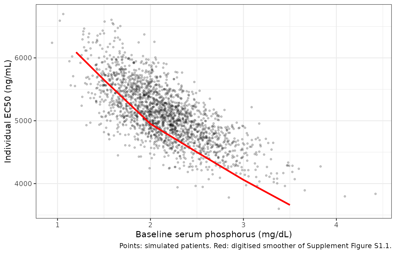
Virtual cohort: UX023-CL303
The cohort follows UX023-CL303, with 200 virtual adults per arm. Body weight is log-normal around a median of 72 kg (log-scale SD 0.22), because the paper does not report weights. The dose is 1.0 mg/kg rounded to the nearest 10 mg, with a 90 mg cap, every 4 weeks. The burosumab arm doses from week 0 to week 112. The placebo arm starts open-label burosumab at week 24. Each subject is followed to week 116 on a daily grid.
rxode2::rxSetSeed(20250101)
n_arm <- 200
cohort <- data.frame(
  id = seq_len(2 * n_arm),
  arm = rep(c("Burosumab", "Placebo"), each = n_arm),
  WT = exp(rnorm(2 * n_arm, log(72), 0.22))
) |>
  dplyr::mutate(
    dose_mg = pmin(90, round(WT / 10) * 10),
    TRT_BUROSUMAB = as.integer(arm == "Burosumab")
  )

wk <- 168
dose_rows <- cohort |>
  dplyr::cross_join(data.frame(dose_wk = seq(0, 112, by = 4))) |>
  dplyr::filter(arm == "Burosumab" | dose_wk >= 24) |>
  dplyr::transmute(id, time = dose_wk * wk, evid = 1L, amt = dose_mg, cmt = "depot", dvid = NA_integer_, WT, arm)
obs_rows <- cohort |>
  dplyr::cross_join(data.frame(time = seq(0, 116 * wk, by = 24))) |>
  # Two endpoints (Cc, serum_phosphorus): observation rows are tagged with
  # dvid = 1 (Cc); serum_phosphorus is returned on the same rows.
  dplyr::transmute(id, time, evid = 0L, amt = 0, cmt = NA_character_, dvid = 1L, WT, arm)
events <- dplyr::bind_rows(dose_rows, obs_rows) |>
  dplyr::arrange(id, time, dplyr::desc(evid))

cohort |>
  dplyr::group_by(arm) |>
  dplyr::summarise(
    N = dplyr::n(),
    `Median WT (kg)` = median(WT),
    `Median dose (mg)` = median(dose_mg),
    `Capped at 90 mg (%)` = 100 * mean(dose_mg == 90)
  ) |>
knitr::kable(digits = 1, caption = "Virtual cohort.")| arm | N | Median WT (kg) | Median dose (mg) | Capped at 90 mg (%) |
|---|---|---|---|---|
| Burosumab | 200 | 72.0 | 70 | 21.5 |
| Placebo | 200 | 72.8 | 70 | 24.5 |
Serum burosumab and serum phosphorus
prof <- sim |>
  dplyr::filter(week %% 1 == 0) |>
  dplyr::select(id, arm, week, Cc, serum_phosphorus) |>
  tidyr::pivot_longer(c(Cc, serum_phosphorus), names_to = "output") |>
  dplyr::mutate(output = dplyr::recode(output,
    Cc = "Serum burosumab (ng/mL)",
    serum_phosphorus = "Serum phosphorus (mg/dL)"
  )) |>
  dplyr::group_by(arm, output, week) |>
  dplyr::summarise(
    med = median(value), lo = quantile(value, 0.05), hi = quantile(value, 0.95),
    .groups = "drop"
  )

ggplot(prof, aes(week, med, colour = arm, fill = arm)) +
  geom_ribbon(aes(ymin = lo, ymax = hi), alpha = 0.2, colour = NA) +
  geom_line() +
  geom_hline(
    data = data.frame(output = "Serum phosphorus (mg/dL)", y = 2.5),
    aes(yintercept = y), linetype = "dashed"
  ) +
  facet_wrap(~output, ncol = 1, scales = "free_y") +
  labs(
    x = "Week", y = NULL, colour = NULL, fill = NULL,
    caption = "Median and 90% prediction interval (individual predictions). Dashed: 2.5 mg/dL lower limit of normal."
  ) +
  theme_bw()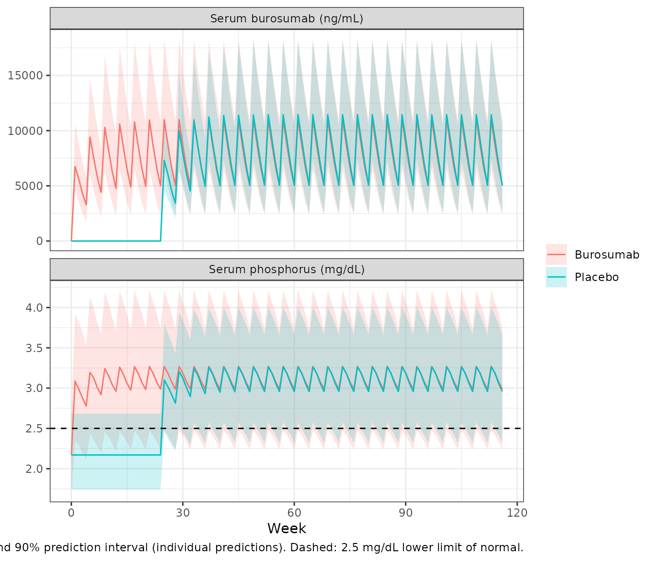
PKNCA: first dose and steady state
Mehta 2025 reports no NCA. The check therefore compares two things.
The first is the simulated AUC over a 4-week interval at steady state.
The second is the closed form dose / CL_i for each subject.
The closed form uses the same drawn parameters, so it isolates the
solver and the unit handling (mg, L, h, ng/mL).
iv_start <- c(first = 0, steady = 108 * wk)
nca_conc <- sim |>
  dplyr::filter(arm == "Burosumab", !is.na(Cc)) |>
  dplyr::select(id, arm, time, Cc)
nca_dose <- dose_rows |>
  dplyr::filter(arm == "Burosumab") |>
  dplyr::select(id, arm, time, amt)

conc_obj <- PKNCA::PKNCAconc(nca_conc, Cc ~ time | arm + id)
dose_obj <- PKNCA::PKNCAdose(nca_dose, amt ~ time | arm + id)
intervals <- data.frame(
  start = iv_start, end = iv_start + 4 * wk,
  cmax = TRUE, tmax = TRUE, auclast = TRUE, cav = TRUE
)
nca_res <- as.data.frame(PKNCA::pk.nca(PKNCA::PKNCAdata(conc_obj, dose_obj, intervals = intervals)))

nca_res |>
  dplyr::mutate(interval = ifelse(start == 0, "Dose 1 (weeks 0-4)", "Steady state (weeks 108-112)")) |>
  dplyr::group_by(interval, PPTESTCD) |>
  dplyr::summarise(median = median(PPORRES), .groups = "drop") |>
  tidyr::pivot_wider(names_from = PPTESTCD, values_from = median) |>
  dplyr::rename(
    "Interval" = interval, "Cmax (ng/mL)" = cmax, "Tmax (h)" = tmax,
    "AUC0-672h (ng*h/mL)" = auclast, "Cav (ng/mL)" = cav
  ) |>
knitr::kable(digits = 0, caption = "Median NCA parameters, burosumab arm.")| Interval | AUC0-672h (ng*h/mL) | Cav (ng/mL) | Cmax (ng/mL) | Tmax (h) |
|---|---|---|---|---|
| Dose 1 (weeks 0-4) | 3381836 | 5032 | 6778 | 168 |
| Steady state (weeks 108-112) | 5563839 | 8280 | 11158 | 120 |
ss_chk <- nca_res |>
  dplyr::filter(start == iv_start[["steady"]], PPTESTCD == "auclast") |>
  dplyr::select(id, auc_nca = PPORRES) |>
  dplyr::left_join(
    sim |> dplyr::distinct(id, cl) |>
      dplyr::left_join(dplyr::select(cohort, id, dose_mg), by = "id"),
    by = "id"
  ) |>
  dplyr::mutate(
    auc_closed = 1000 * dose_mg / cl,
    pct_diff = 100 * (auc_nca / auc_closed - 1)
  )

# Same drawn parameters on both sides. The remaining gap is the linear
# trapezoid on a daily grid plus residual accumulation (t1/2 ~ 18 days, so
# after 27 doses steady state is complete to well under 1%).
stopifnot(
  nrow(ss_chk) == n_arm,
  abs(median(ss_chk$pct_diff)) < 2,
  quantile(abs(ss_chk$pct_diff), 0.9) < 3
)
The median steady-state AUC differs from dose / CL by
-0.13%.
Per-cycle average serum phosphorus
The authors calculated the “average … serum phosphate concentrations
per dosing cycle” from the individual PK/PD predictions and matched them
in time to the fracture surveys. Here, each survey at week
v > 0 takes the mean serum phosphorus over the 4-week
cycle that ends at v, [v - 4, v). The week-0
survey is before the first dose, so it takes the patient’s baseline
e0. The paper does not state which cycle was matched to
each survey.
visits <- c(0, 12, 24, 36, 48, 84, 96, 108, 116)
cav <- sim |>
  dplyr::select(id, arm, week, serum_phosphorus) |>
  dplyr::cross_join(data.frame(visit = visits)) |>
  dplyr::filter(
    (visit == 0 & week == 0) | (visit > 0 & week >= visit - 4 & week < visit)
  ) |>
  dplyr::group_by(id, arm, visit) |>
  dplyr::summarise(cav_mgdl = mean(serum_phosphorus), .groups = "drop")

cav |>
  dplyr::group_by(arm, visit) |>
  dplyr::summarise(
    median = median(cav_mgdl),
    pct_ge_2.5 = 100 * mean(cav_mgdl >= 2.5),
    .groups = "drop"
  ) |>
  tidyr::pivot_wider(names_from = arm, values_from = c(median, pct_ge_2.5)) |>
  dplyr::rename(
    "Week" = visit,
    "Median Cavg, burosumab (mg/dL)" = median_Burosumab,
    "Median Cavg, placebo (mg/dL)" = median_Placebo,
    "Cavg >= 2.5, burosumab (%)" = pct_ge_2.5_Burosumab,
    "Cavg >= 2.5, placebo (%)" = pct_ge_2.5_Placebo
  ) |>
knitr::kable(digits = 2, caption = "Per-cycle average serum phosphorus at each fracture survey.")| Week | Median Cavg, burosumab (mg/dL) | Median Cavg, placebo (mg/dL) | Cavg >= 2.5, burosumab (%) | Cavg >= 2.5, placebo (%) |
|---|---|---|---|---|
| 0 | 2.17 | 2.17 | 12.5 | 16 |
| 12 | 3.11 | 2.17 | 90.0 | 16 |
| 24 | 3.14 | 2.17 | 91.0 | 16 |
| 36 | 3.14 | 3.12 | 91.5 | 93 |
| 48 | 3.14 | 3.14 | 91.5 | 93 |
| 84 | 3.14 | 3.15 | 91.5 | 93 |
| 96 | 3.14 | 3.15 | 91.5 | 93 |
| 108 | 3.14 | 3.15 | 91.5 | 93 |
| 116 | 3.14 | 3.15 | 91.5 | 93 |
Fracture and pseudofracture counts
The cycle averages, converted to mmol/L, are passed to the fracture
model with the randomised-arm indicator. The model output
fracture_count is the Poisson mean, and counts are drawn
from it with rpois().
fx_events <- cav |>
  dplyr::left_join(dplyr::select(cohort, id, TRT_BUROSUMAB), by = "id") |>
  dplyr::transmute(
    id, time = visit, evid = 0L, amt = 0, arm,
    CAV_PHOS = cav_mgdl / 3.0975, TRT_BUROSUMAB
  ) |>
  dplyr::arrange(id, time)

fx_sim <- rxode2::rxSolve(fx, fx_events, keep = "arm", returnType = "data.frame") |>
  dplyr::select(-dplyr::any_of("CAV_PHOS")) |>
  dplyr::left_join(dplyr::select(fx_events, id, time, CAV_PHOS), by = c("id", "time"))
set.seed(116)
fx_sim$count <- rpois(nrow(fx_sim), fx_sim$fracture_count)
Means by arm and visit (Table 3)
Table 3 gives the observed mean count by arm and visit. The comparison below puts the simulated mean count next to it, and both counts relative to week 0. The relative scale removes the base-rate offset between arms.
tab3 <- data.frame(
  visit = rep(visits, 2),
  arm = rep(c("Burosumab", "Placebo"), each = length(visits)),
  obs = c(
    2.03, 1.59, 1.10, 1.00, 0.77, 0.86, 0.56, 0.55, 0.40,
    2.39, 2.32, 2.18, 1.82, 1.24, 1.20, 0.94, 0.93, 0.73
  )
)
cmp3 <- fx_sim |>
  dplyr::group_by(arm, visit = time) |>
  dplyr::summarise(pred = mean(fracture_count), .groups = "drop") |>
  dplyr::left_join(tab3, by = c("arm", "visit")) |>
  dplyr::group_by(arm) |>
  dplyr::mutate(
    pred_rel = pred / pred[visit == 0],
    obs_rel = obs / obs[visit == 0]
  ) |>
  dplyr::ungroup()

cmp3 |>
  dplyr::select(arm, visit, obs, pred, obs_rel, pred_rel) |>
  dplyr::rename(
    "Arm" = arm, "Week" = visit, "Observed mean (Table 3)" = obs,
    "Simulated mean" = pred, "Observed / week 0" = obs_rel, "Simulated / week 0" = pred_rel
  ) |>
knitr::kable(digits = 2, caption = "Simulated against observed mean counts (Table 3 of Mehta 2025).")| Arm | Week | Observed mean (Table 3) | Simulated mean | Observed / week 0 | Simulated / week 0 |
|---|---|---|---|---|---|
| Burosumab | 0 | 2.03 | 2.13 | 1.00 | 1.00 |
| Burosumab | 12 | 1.59 | 1.44 | 0.78 | 0.68 |
| Burosumab | 24 | 1.10 | 1.25 | 0.54 | 0.59 |
| Burosumab | 36 | 1.00 | 1.08 | 0.49 | 0.51 |
| Burosumab | 48 | 0.77 | 0.94 | 0.38 | 0.44 |
| Burosumab | 84 | 0.86 | 0.62 | 0.42 | 0.29 |
| Burosumab | 96 | 0.56 | 0.54 | 0.28 | 0.25 |
| Burosumab | 108 | 0.55 | 0.47 | 0.27 | 0.22 |
| Burosumab | 116 | 0.40 | 0.43 | 0.20 | 0.20 |
| Placebo | 0 | 2.39 | 2.17 | 1.00 | 1.00 |
| Placebo | 12 | 2.32 | 2.02 | 0.97 | 0.93 |
| Placebo | 24 | 2.18 | 1.89 | 0.91 | 0.87 |
| Placebo | 36 | 1.82 | 1.38 | 0.76 | 0.64 |
| Placebo | 48 | 1.24 | 1.28 | 0.52 | 0.59 |
| Placebo | 84 | 1.20 | 1.04 | 0.50 | 0.48 |
| Placebo | 96 | 0.94 | 0.97 | 0.39 | 0.45 |
| Placebo | 108 | 0.93 | 0.91 | 0.39 | 0.42 |
| Placebo | 116 | 0.73 | 0.86 | 0.31 | 0.40 |
rel <- function(a, v) cmp3$pred_rel[cmp3$arm == a & cmp3$visit == v] / cmp3$obs_rel[cmp3$arm == a & cmp3$visit == v]
# Arm-level means of 200 subjects; the relative change is driven by the
# fixed-effect time and phosphorus terms, so a mis-transcribed slope or a
# unit slip in CAV_PHOS shifts it by far more than 30%.
stopifnot(
  abs(log(rel("Burosumab", 116))) < log(1.3),
  abs(log(rel("Placebo", 24))) < log(1.3)
)
In the burosumab arm, the simulated change from week 0 follows the observed means to week 116 (0.20 of baseline on both sides). The placebo arm crossed over at week 24. From then on, the static randomised-arm coding gives it the phosphorus benefit but not the extra burosumab time effect. Its simulated count drops more steeply than observed just after crossover (week 36). By week 116 it sits above the observed mean (about 0.40 against 0.31 of baseline).
Visual predictive check (Figure 1)
vpc <- fx_sim |>
  dplyr::filter(arm == "Burosumab" | time <= 24) |>
  dplyr::group_by(arm, time) |>
  dplyr::summarise(
    mean = mean(count),
    lo = quantile(count, 0.25), hi = quantile(count, 0.75),
    .groups = "drop"
  )

ggplot(vpc, aes(time, mean)) +
  geom_ribbon(aes(ymin = lo, ymax = hi), fill = "grey80") +
  geom_line() +
  geom_line(
    data = dplyr::filter(tab3, arm == "Burosumab" | visit <= 24),
    aes(visit, obs), colour = "blue"
  ) +
  facet_wrap(~arm, scales = "free_x") +
  labs(
    x = "Time (weeks)", y = "Total fractures and pseudofractures",
    caption = "Black: simulated mean count; grey: simulated interquartile range; blue: observed mean (Table 3)."
  ) +
  theme_bw()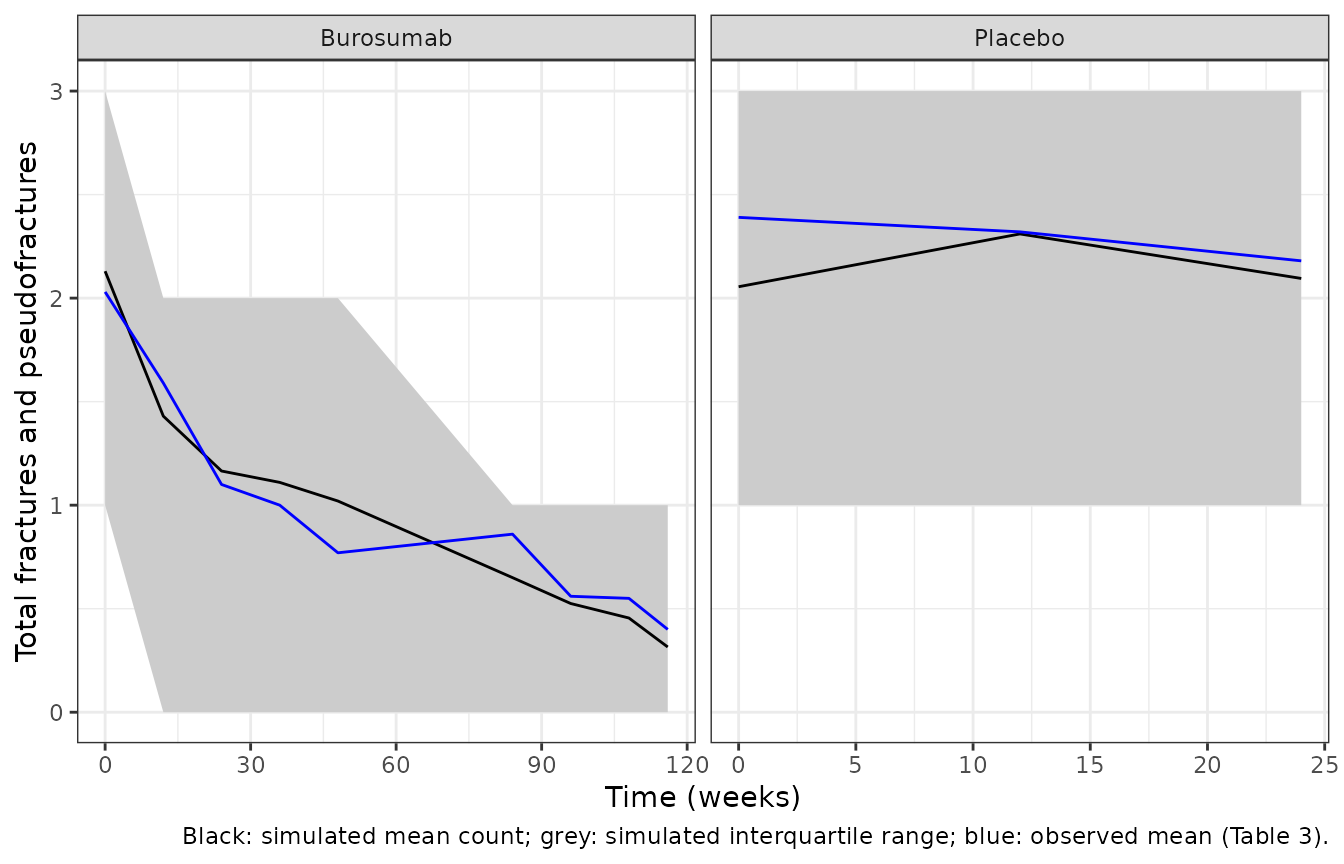
Replicates Figure 1 of Mehta 2025. The figure shows the placebo arm only during the double-blind period, as the paper does. The paper plots medians and a 95% interval of the simulated median. Only means are printed (Table 3), so this version plots means.
Individual predictions by serum phosphorus group (Figure 2)
set.seed(2)
show_ids <- c(
  sample(cohort$id[cohort$arm == "Burosumab"], 25),
  sample(cohort$id[cohort$arm == "Placebo"], 25)
)
fig2 <- fx_sim |>
  dplyr::filter(id %in% show_ids, time <= 84) |>
  dplyr::mutate(group = ifelse(CAV_PHOS * 3.0975 >= 2.5, ">=2.5", "<2.5"))

ggplot(fig2, aes(time, fracture_count, group = id)) +
  geom_line(aes(colour = group)) +
  facet_wrap(~ factor(arm, levels = c("Placebo", "Burosumab"))) +
  labs(
    x = "Time (weeks)", y = "Predicted fractures and pseudofractures",
    colour = "Average serum phosphate\nper cycle (mg/dL)"
  ) +
  theme_bw() +
  theme(legend.position = "bottom")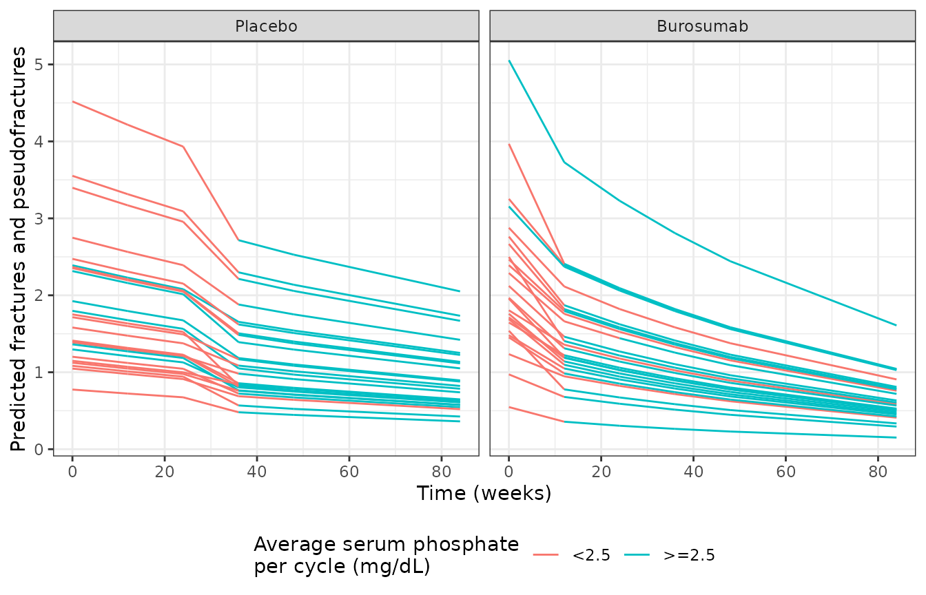
Replicates Figure 2 of Mehta 2025: individual predicted mean counts, coloured by the cycle-average serum phosphorus at each survey. The colour is drawn per point, so a line can change colour between surveys. The published week-0 predictions are whole numbers, which suggests the published figure shows each patient’s observed baseline count at week 0. Here, week 0 shows the model prediction.
Discussion scenarios: 24 weeks at 2.5 or 3.5 mg/dL
The Discussion states that 24 weeks of burosumab with the average serum phosphorus held at about 2.5 or 3.5 mg/dL reduces the fracture count from baseline by about 48% and 74%. The Table 4 estimates give the following:
bl_cav <- exp(th[["le0"]])
scen <- data.frame(cav = c(2.5, 3.5)) |>
  dplyr::mutate(
    from_bsl = 100 * (1 - exp(
      (th[["e_time_base"]] + th[["e_trt_time_base"]]) * 24 +
        th[["e_cavphos_base"]] * (cav - bl_cav)
    )),
    from_llnorm = 100 * (1 - exp(
      (th[["e_time_base"]] + th[["e_trt_time_base"]]) * 24 +
        th[["e_cavphos_base"]] * (cav - 2.5)
    )),
    paper = c(48, 74)
  )
scen |>
  dplyr::rename(
    "Cavg held at (mg/dL)" = cav,
    "Reduction vs baseline at BSL 2.14 mg/dL (%)" = from_bsl,
    "Reduction vs baseline at 2.5 mg/dL (%)" = from_llnorm,
    "Discussion (%)" = paper
  ) |>
knitr::kable(digits = c(1, 0, 0, 0), caption = "Week-24 reduction from baseline under the Table 4 estimates.")| Cavg held at (mg/dL) | Reduction vs baseline at BSL 2.14 mg/dL (%) | Reduction vs baseline at 2.5 mg/dL (%) | Discussion (%) |
|---|---|---|---|
| 2.5 | 31 | 24 | 48 |
| 3.5 | 47 | 42 | 74 |
Neither reading of the baseline reproduces the 48% and 74% in the Discussion. The model is not tuned to them. The gap is listed under Assumptions and deviations.
Assumptions and deviations
-
Form of
dEC50dBPHOS. The paper does not print it. The maintainers adoptedEC50 = 8270 * e0_i^-0.64, an uncentred power function of the model’s individual baseline. This is the only form among those tried that reproduces the level and slope of Supplement Figure S1.1 and the figure’s vertical scatter, since EC50 carries no IIV. - Reference weight. Not printed. 70 kg is used, as in Lee 2022, whose dataset this analysis extends.
- Additive PK error unit. Table 2 prints ‘ng/L’ for the additive error of 39.32. It is read as ng/mL, the assay unit (LLOQ 36-50 ng/mL).
-
Combined residual error form. Not printed. The
Pumas convention
SD = sqrt(add^2 + (prop * Cc)^2)(combined2) is used. -
CV to variance. The IIV percentages in Tables 2 and
4 are read as CVs of log-normal parameters,
omega^2 = log(CV^2 + 1). The Results text gives the IIV on the fracture base rate as “approximately 40%”, against 45.15% in Table 4. The table value is used. - Identical alpha and beta rows. Table 4 prints the same estimate, RSE and bootstrap CI for tv-alpha and tv-beta (-0.0058; CI -0.0078 to 0.0039). Both are used as printed. The Abstract describes each as about 1% per week, while -0.0058 is 0.58% per week.
- Discussion scenarios. The 48% and 74% reductions in the Discussion do not follow from Table 4 under either baseline reading (see above).
-
Treatment indicator after crossover. The paper does
not state how the indicator was coded once the placebo arm crossed over
at week 24. The maintainers adopted the static randomised arm
(
TRT_BUROSUMAB = 0throughout for placebo-randomised patients). Their post-crossover benefit therefore enters only through serum phosphorus. -
Cycle matching. Each survey uses the average over
the 4-week cycle ending at the survey, and the baseline survey uses the
model baseline
e0. The paper says only that the cycle averages were “merged with individual time-matched fracture and pseudofracture count data”. - Centre of the phosphorus effect. 2.5 mg/dL, from the Abstract and Discussion. Table 4 does not print the centre.
- Cohort. Body weight is assumed log-normal with a median of 72 kg. The simulated cohort uses 200 patients per arm and includes no dropouts. The analysed patients all had at least one fracture at baseline, and that selection is reflected only through the fitted base rate.
- Erratum check. On 2026-11-02 a Europe PMC search found no correction notice for this article.