NLG207 conjugated and free camptothecin (Schmidt 2020)
Source:vignettes/articles/Schmidt_2020_camptothecin.Rmd
Schmidt_2020_camptothecin.RmdModel and source
mod <- rxode2::rxode2(readModelDb("Schmidt_2020_camptothecin"))
#> ℹ parameter labels from comments will be replaced by 'label()'
mod_typ <- rxode2::zeroRe(mod)- Citation: Schmidt KT, Huitema ADR, Dorlo TPC, Peer CJ, Cordes LM, Sciuto L, Wroblewski S, Pommier Y, Madan RA, Thomas A, Figg WD. Population pharmacokinetic analysis of nanoparticle-bound and free camptothecin after administration of NLG207 in adults with advanced solid tumors. Cancer Chemother Pharmacol. 2020;86(4):475-486. doi:10.1007/s00280-020-04134-9. PMCID: PMC7515962.
- Article: https://doi.org/10.1007/s00280-020-04134-9
- PubMed Central (open access): https://www.ncbi.nlm.nih.gov/pmc/articles/PMC7515962/
NLG207 (formerly CRLX101) is a nanoparticle-drug conjugate in which the topoisomerase-I inhibitor camptothecin (CPT) is covalently linked to a cyclodextrin-containing polymer that self-assembles into nanoparticles. CPT is released from the polymer by hydrolysis. Schmidt 2020 measured nanoparticle-bound (conjugated) and free CPT in the same plasma samples and fit both together in NONMEM (FOCE-I, ADVAN13):
-
Conjugated CPT (
central_np,peripheral1_np; outputCc_np) follows a linear two-compartment model. Its only route out of the body is conversion to free CPT in the central compartment. -
The release clearance is the sum of two parts
(Figure 1). One is a steady-state part,
CL_B. The other is a fast part,CL_F, that decays mono-exponentially with time after the start of each infusion:CL1 = CL_B + CL_F * exp(-(ln 2 / t1/2) * t). -
Free CPT (
central,peripheral1; outputCc) follows a second linear two-compartment model with first-order elimination (CL3). The fraction of conjugated CPT that ends up as free CPT is not identifiable, so the free-CPT volumes and clearances are apparent values relative to that fraction.
All clearances and volumes except CL_F and
t1/2 are scaled allometrically on body weight, with fixed
exponents (1 for volumes, 0.75 for clearances) and a reference weight of
70 kg.
The _np suffix follows the library’s nanoparticle
convention: the bare compartment and output names hold the free
(released) drug, and the _np suffix holds the drug that is
still conjugated.
Population
| Field | Value |
|---|---|
| Subjects | 27 |
| Studies | 2 |
| Observations | 477 |
| Age | 60 years (47-76 years) |
| Weight | 70.4 kg (46.4-105 kg) |
| Female | 55.6% |
| Race | Caucasian 74.1%, African 14.8%, Asian 11.1% |
| Disease | Advanced solid tumours (NSCLC, small cell, pancreatic, cholangiocarcinoma, ovarian/fallopian tube, mCRPC, cervical, colorectal, mesothelioma, myxofibrosarcoma, thymic) |
| Dosing | NLG207 12 mg/m^2 IV over 1 or 2 h every 2 weeks at cycle 1 (two cycle-6 patients dose-reduced to 50% and 75%) |
There were 27 adults with advanced solid tumours in two phase II trials at the US National Cancer Institute: NCT02769962 (NLG207 plus olaparib, n = 24) and NCT03531827 (NLG207 plus enzalutamide, n = 3). All received NLG207 12 mg/m^2 IV over 1 or 2 h at cycle 1. Dense samples were taken up to 24 or 48 h after the end of infusion, plus a sample at about 14 to 16 days in NCT02769962. Five patients were sampled again at cycle 6. Cycle-1 samples were collected before the combination partner was given.
Source trace
| Model element | Value | Source |
|---|---|---|
| Structure: 2-cmt conjugated + 2-cmt free CPT, release only from conjugated central | – | Methods ‘Pharmacokinetic model-building procedure’; Fig. 1 |
CL1 = CL_B + CL_F * exp(-(ln 2 / t1/2) * t) |
– | Fig. 1 equation |
Time origin of t = start of each infusion |
– | Discussion (release half-life 0.38 h at start of infusion, 22 h at 4 h) |
lvc_np (V1, 70 kg) |
3.16 L | Table 2 |
lvp_np (V2, 70 kg) |
2.09 L | Table 2 |
lq_np (Q1, 70 kg) |
0.0482 L/h | Table 2 |
lcl_exp_inf_np (CL_B, 70 kg) |
0.0988 L/h | Table 2 |
lcl_exp_component_np (CL_F) |
5.71 L/h | Table 2 |
lcl_exp_kdes_np |
ln(2)/0.307 = 2.258 1/h | Table 2 (t1/2 = 0.307 h) |
lvc (V3, 70 kg) |
21.1 L | Table 2 |
lvp (V4, 70 kg) |
19.4 L | Table 2 |
lq (Q3, 70 kg) |
25.6 L/h | Table 2 |
lcl (CL3, 70 kg) |
0.874 L/h | Table 2 |
e_wt_vc_vp, e_wt_cl_q
|
1, 0.75 (fixed) | Table 2 formulas; Results ‘Covariate model’ |
etalvc_np, etalcl_exp_inf_np (block) |
CV 18.1%, 33.5%; r = 0.918 | Table 2 |
etalcl_exp_component_np |
CV 62.6% | Table 2 |
etalvc, etalcl (block) |
CV 79.8%, 42.2%; r = 0.884 | Table 2 |
propSd_np, addSd_np
|
12.3%, 5.07 ng/mL | Table 2 ‘BoundRE’ |
propSd, addSd
|
24.8%, 0.396 ng/mL | Table 2 ‘FreeRE’ |
Residual form C * (1 + eps_prop) + eps_add
|
– | Methods Eq. 2 |
Deterministic checks against the paper’s derived quantities
The paper does not report an NCA table. Its Discussion does quote several quantities that follow directly from the typical parameters, and each one can be recomputed without any random draw. The first three check the release clearance, and the last two check the free-CPT disposition parameters.
th <- mod$theta
v1 <- exp(th[["lvc_np"]])
clb <- exp(th[["lcl_exp_inf_np"]])
clf <- exp(th[["lcl_exp_component_np"]])
kdes <- exp(th[["lcl_exp_kdes_np"]])
cl1 <- function(t) clb + clf * exp(-kdes * t)
release_hl <- function(t) log(2) * v1 / cl1(t)

biexp_hl <- function(cl, v1, q, v2) {
  k10 <- cl / v1
  k12 <- q / v1
  k21 <- q / v2
  s <- k10 + k12 + k21
  d <- sqrt(s^2 - 4 * k10 * k21)
  c(alpha = log(2) / ((s + d) / 2), beta = log(2) / ((s - d) / 2))
}
hl_free <- biexp_hl(
  exp(th[["lcl"]]), exp(th[["lvc"]]), exp(th[["lq"]]), exp(th[["lvp"]])
)

derived <- tibble::tribble(
  ~Quantity, ~Model, ~Published,
  "Release half-life at start of infusion (h)", release_hl(0), 0.38,
  "Release half-life at 4 h after start (h)", release_hl(4), 22,
  "CL_F contribution / CL_B at 1.8 h", clf * exp(-kdes * 1.8) / clb, 1,
  "Free CPT distribution half-life (min)", 60 * hl_free[["alpha"]], 16,
  "Free CPT terminal half-life (h)", hl_free[["beta"]], 32.4
) |>
  dplyr::mutate(`% diff` = 100 * (.data$Model - .data$Published) / .data$Published)

derived |>
  dplyr::mutate(Model = signif(.data$Model, 3), `% diff` = round(.data$`% diff`, 1)) |>
knitr::kable(caption = "Typical-value quantities quoted in the Schmidt 2020 Discussion.")| Quantity | Model | Published | % diff |
|---|---|---|---|
| Release half-life at start of infusion (h) | 0.377 | 0.38 | -0.8 |
| Release half-life at 4 h after start (h) | 22.000 | 22.00 | 0.1 |
| CL_F contribution / CL_B at 1.8 h | 0.993 | 1.00 | -0.7 |
| Free CPT distribution half-life (min) | 16.300 | 16.00 | 1.8 |
| Free CPT terminal half-life (h) | 32.400 | 32.40 | -0.1 |
# Deterministic: no random effects are involved, so a tight bound is correct.
# The published values are rounded to 2-3 significant figures ("~16 min",
# "near equal contribution").
stopifnot(all(abs(derived$`% diff`) < 5))
All five agree to within the rounding of the published text. The 0.38
h and 22 h release half-lives pin both the release equation and its time
origin at the start of the infusion. If t were measured
from the end of a 1 h infusion instead, the half-life at 4 h after the
start would be about 21 h, not 22 h.
Typical-subject profile and mass balance
The typical 70 kg subject has a BSA of about 1.8 m^2, so a 12 mg/m^2 dose over 1 h is about 21.6 mg of CPT.
make_events <- function(subjects, obs_times, n_doses = 1L) {
  dose_times <- (seq_len(n_doses) - 1) * 336
  doses <- tidyr::crossing(subjects, time = dose_times) |>
    dplyr::mutate(
      amt = .data$dose_mg, evid = 1L, cmt = "central_np",
      dur = .data$tinf, dvid = NA_integer_
    )
  obs <- tidyr::crossing(subjects, time = obs_times) |>
    dplyr::mutate(amt = 0, evid = 0L, cmt = NA_character_, dur = NA_real_, dvid = 1L)
  dplyr::bind_rows(doses, obs) |>
    dplyr::arrange(.data$id, .data$time, dplyr::desc(.data$evid)) |>
    dplyr::select("id", "time", "amt", "evid", "cmt", "dur", "dvid", dplyr::everything()) |>
    as.data.frame()
}

typ_subject <- data.frame(id = 1L, WT = 70, dose_mg = 12 * 1.8, tinf = 1)
obs_fine <- sort(unique(c(seq(0, 4, by = 0.05), seq(4.25, 48, by = 0.25), seq(49, 2000, by = 1))))
sim_typ <- rxode2::rxSolve(
  mod_typ, make_events(typ_subject, obs_fine),
  returnType = "data.frame"
)
#> ℹ omega/sigma items treated as zero: 'etalvc_np', 'etalcl_exp_inf_np', 'etalcl_exp_component_np', 'etalvc', 'etalcl'
sim_typ |>
  dplyr::filter(.data$time <= 96) |>
  dplyr::select("time", "Conjugated CPT" = "Cc_np", "Free CPT" = "Cc") |>
  tidyr::pivot_longer(-"time", names_to = "Analyte", values_to = "conc") |>
  dplyr::filter(.data$conc > 0) |>
  ggplot(aes(.data$time, .data$conc, colour = .data$Analyte)) +
  geom_line() +
  scale_y_log10() +
  labs(x = "Time after start of infusion (h)", y = "Concentration (ng/mL)", colour = NULL)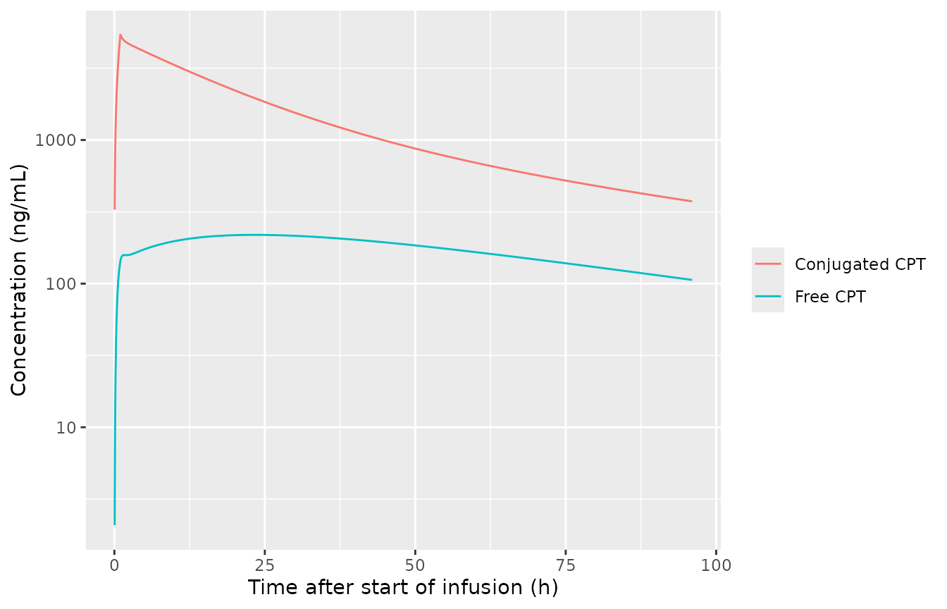
Typical-subject conjugated and free CPT after 12 mg/m^2 over 1 h (70 kg, BSA 1.8 m^2).
Conjugated CPT has no elimination route other than release, so every
milligram dosed eventually leaves the body as free CPT through
CL3. The dose must therefore equal
CL3 * AUC(0-inf) of free CPT. This check is exact, and it
would fail if the release flux were lost or double-counted between the
two sub-models.
cl3_typ <- exp(th[["lcl"]])
auc_free <- with(
  dplyr::filter(sim_typ, !is.na(.data$Cc)),
  sum(diff(time) * (head(Cc, -1) + tail(Cc, -1)) / 2)
)
# Remaining tail beyond the last point, using the conjugated terminal slope that
# governs the free-CPT decline at late times.
tail_end <- tail(sim_typ, 2)
lz <- log(tail_end$Cc[1] / tail_end$Cc[2]) / diff(tail_end$time)
auc_free_inf <- auc_free + tail(sim_typ$Cc, 1) / lz
recovered_mg <- cl3_typ * auc_free_inf / 1000 # L/h * ng.h/mL = ug -> mg
c(dose_mg = typ_subject$dose_mg, recovered_mg = recovered_mg)
#>      dose_mg recovered_mg
#>      21.6000      21.6001
stopifnot(abs(recovered_mg / typ_subject$dose_mg - 1) < 0.005)
The model also has to reset the release clock at each dose, since
each infusion delivers fresh nanoparticles. The release clearance should
return to CL_B + CL_F at the start of cycle 2 (336 h).
sim_2 <- rxode2::rxSolve(
  mod_typ, make_events(typ_subject, c(0, 1, 4, 336, 337, 340), n_doses = 2L),
  returnType = "data.frame"
)
#> ℹ omega/sigma items treated as zero: 'etalvc_np', 'etalcl_exp_inf_np', 'etalcl_exp_component_np', 'etalvc', 'etalcl'
sim_2 |> dplyr::select("time", "cl_release") |> knitr::kable(digits = 4)| time | cl_release |
|---|---|
| 0 | 5.8088 |
| 1 | 0.6959 |
| 4 | 0.0995 |
| 336 | 5.8088 |
| 337 | 0.6959 |
| 340 | 0.0995 |
Percent free CPT
The paper reports observed mean (SEM) percent free CPT (free / total). It was 3.13 +/- 0.21% in samples taken within 3 h of the start of infusion, and it rose to 20.42 +/- 0.44% by about 50 h after the dose. These are summaries of observed data rather than model outputs, so they serve as a loose external check.
pct_free <- sim_typ |>
  dplyr::filter(.data$time > 0) |>
  dplyr::mutate(pct = 100 * .data$Cc / (.data$Cc + .data$Cc_np))
early <- mean(pct_free$pct[pct_free$time <= 3])
at50 <- pct_free$pct[pct_free$time == 50]
c(early_0_3h = early, at_50h = at50)
#> early_0_3h     at_50h
#>   2.927461  17.470771
stopifnot(abs(early - 3.13) < 1, abs(at50 - 20.42) / 20.42 < 0.25)
The typical subject gives about 2.9% free CPT over the first 3 h and 17.5% at 50 h. The observed values are 3.13% and 20.42%. The 50 h value is about 15% lower in the model. Two things contribute to that gap: the observed figure is a mean of per-sample ratios over a skewed population, and at 50 h free CPT carries the largest between-subject variability in the model (V3 CV 79.8%).
Virtual cohort and VPC
The cohort has 100 subjects per infusion duration. Body weight is log-normal around the cohort median of 70.4 kg and is redrawn until it falls inside the observed 46.4-105 kg range. Sex is 55.6% female. Height is drawn by sex and is used only to compute a Mosteller BSA for the per-m^2 dose.
n_per_arm <- 100L
draw_wt <- function(n) {
  out <- numeric(0)
  while (length(out) < n) {
    w <- exp(rnorm(n, log(70.4), 0.22))
    out <- c(out, w[w >= 46.4 & w <= 105])
  }
  out[seq_len(n)]
}
cohort <- tibble::tibble(
  id = seq_len(2L * n_per_arm),
  arm = rep(c("12 mg/m^2 over 1 h", "12 mg/m^2 over 2 h"), each = n_per_arm),
  tinf = rep(c(1, 2), each = n_per_arm),
  WT = draw_wt(2L * n_per_arm),
  female = rbinom(2L * n_per_arm, 1, 0.556),
  HT = ifelse(female == 1, rnorm(2L * n_per_arm, 162, 7), rnorm(2L * n_per_arm, 176, 7)),
  BSA = sqrt(HT * WT / 3600),
  dose_mg = 12 * BSA
)
summary(cohort[, c("WT", "BSA", "dose_mg")])
#>        WT              BSA           dose_mg
#>  Min.   : 46.56   Min.   :1.433   Min.   :17.20
#>  1st Qu.: 62.65   1st Qu.:1.696   1st Qu.:20.35
#>  Median : 70.09   Median :1.825   Median :21.90
#>  Mean   : 71.78   Mean   :1.828   Mean   :21.93
#>  3rd Qu.: 82.02   3rd Qu.:1.960   3rd Qu.:23.52
#>  Max.   :102.95   Max.   :2.275   Max.   :27.30
obs_vpc <- sort(unique(c(0, 0.25, 0.5, 0.75, 1, 1.5, 2, 2.5, 3, 4, 5, 6, 8, 10, 12, 16, 24, 36, 48, 50)))
sim_cohort <- rxode2::rxSolve(
  mod, make_events(dplyr::select(cohort, "id", "arm", "WT", "dose_mg", "tinf"), obs_vpc),
  keep = "arm", returnType = "data.frame"
)
vpc_df <- sim_cohort |>
  dplyr::select("id", "arm", "time", "Conjugated CPT" = "Cc_np", "Free CPT" = "Cc") |>
  tidyr::pivot_longer(c("Conjugated CPT", "Free CPT"), names_to = "Analyte", values_to = "conc") |>
  dplyr::filter(.data$time > 0) |>
  dplyr::group_by(.data$arm, .data$Analyte, .data$time) |>
  dplyr::summarise(
    lo = quantile(.data$conc, 0.025), med = median(.data$conc),
    hi = quantile(.data$conc, 0.975), .groups = "drop"
  )
ggplot(vpc_df, aes(.data$time, .data$med, colour = .data$arm, fill = .data$arm)) +
  geom_ribbon(aes(ymin = .data$lo, ymax = .data$hi), alpha = 0.2, colour = NA) +
  geom_line() +
  scale_y_log10() +
  facet_wrap(~Analyte, ncol = 1, scales = "free_y") +
  labs(x = "Time after start of infusion (h)", y = "Concentration (ng/mL)", colour = NULL, fill = NULL)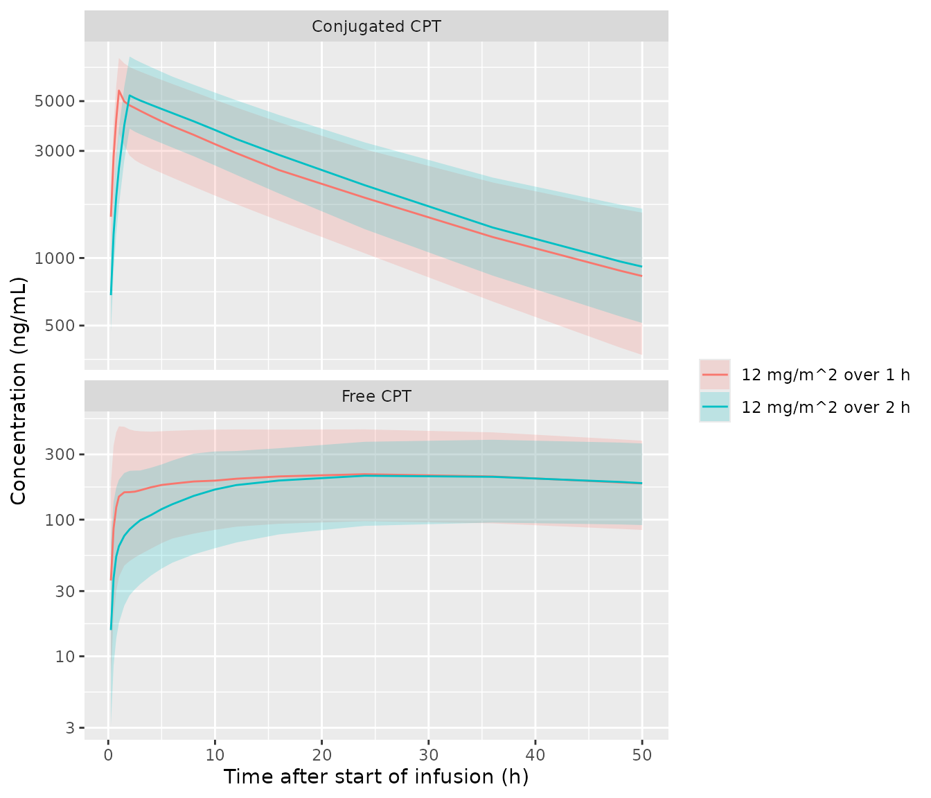
Replicates the layout of Figure 3 of Schmidt 2020: simulated 2.5th, 50th and 97.5th percentiles of conjugated (a) and free (b) CPT up to 50 h. The shading is the 95% prediction interval of individual predictions, without residual error.
Over the whole sampling window, conjugated CPT stays well above free CPT. For the typical subject it is about 35-fold higher at the end of a 1 h infusion, and the gap narrows to about 5-fold by 48 h. Free CPT peaks late, well after the end of infusion. Both features match the paper’s description of Figure 3 and its conclusion that the formulation holds on to most of the CPT during the first 48 h.
PKNCA
The NCA below covers cycle 1 (0 to 336 h) for both analytes, grouped by infusion-duration arm.
obs_nca <- sort(unique(c(obs_vpc, 72, 96, 120, 168, 240, 336)))
sim_nca <- rxode2::rxSolve(
  mod, make_events(dplyr::select(cohort, "id", "arm", "WT", "dose_mg", "tinf"), obs_nca),
  keep = "arm", returnType = "data.frame"
)
dose_df <- cohort |>
  dplyr::transmute(id = .data$id, treatment = .data$arm, time = 0, amt = .data$dose_mg) |>
  as.data.frame()

run_nca <- function(column) {
  conc_df <- sim_nca |>
    dplyr::transmute(id = .data$id, treatment = .data$arm, time = .data$time, conc = .data[[column]]) |>
    dplyr::filter(!is.na(.data$conc)) |>
    as.data.frame()
  conc_obj <- PKNCA::PKNCAconc(conc_df, conc ~ time | treatment + id, concu = "ng/mL", timeu = "h")
  dose_obj <- PKNCA::PKNCAdose(dose_df, amt ~ time | treatment + id, doseu = "mg")
  intervals <- data.frame(start = 0, end = 336, cmax = TRUE, tmax = TRUE, auclast = TRUE, half.life = TRUE)
  res <- PKNCA::pk.nca(PKNCA::PKNCAdata(conc_obj, dose_obj, intervals = intervals))
  as.data.frame(res) |>
    dplyr::filter(.data$PPTESTCD %in% c("cmax", "tmax", "auclast", "half.life")) |>
    dplyr::group_by(.data$treatment, .data$PPTESTCD) |>
    dplyr::summarise(median = median(.data$PPORRES, na.rm = TRUE), .groups = "drop") |>
    tidyr::pivot_wider(names_from = "PPTESTCD", values_from = "median")
}
nca_np <- run_nca("Cc_np") |> dplyr::mutate(Analyte = "Conjugated CPT", .before = 1)
nca_free <- run_nca("Cc") |> dplyr::mutate(Analyte = "Free CPT", .before = 1)
nca_all <- dplyr::bind_rows(nca_np, nca_free)
nca_all |>
  dplyr::rename(
    "Arm" = "treatment", "Cmax (ng/mL)" = "cmax", "Tmax (h)" = "tmax",
    "AUC0-336 (ng*h/mL)" = "auclast", "t1/2 (h)" = "half.life"
  ) |>
knitr::kable(digits = 3, caption = "Median simulated cycle-1 NCA by analyte and infusion duration.")| Analyte | Arm | AUC0-336 (ng*h/mL) | Cmax (ng/mL) | t1/2 (h) | Tmax (h) |
|---|---|---|---|---|---|
| Conjugated CPT | 12 mg/m^2 over 1 h | 155699.67 | 5142.299 | 53.297 | 1 |
| Conjugated CPT | 12 mg/m^2 over 2 h | 179824.70 | 5385.226 | 53.580 | 2 |
| Free CPT | 12 mg/m^2 over 1 h | 23899.53 | 217.138 | 54.738 | 24 |
| Free CPT | 12 mg/m^2 over 2 h | 24133.88 | 191.254 | 58.595 | 36 |
free_tmax <- nca_free$tmax
np_hl <- nca_np$half.life
stopifnot(
  # Free CPT peaks well after the end of infusion (delayed Cmax; paper Results).
  all(free_tmax > 6),
  # The free-CPT terminal decline follows the release-limited conjugated
  # terminal phase (~55 h for the typical subject), not the 32.4 h disposition
  # half-life of free CPT itself.
  all(abs(nca_free$half.life / np_hl - 1) < 0.15),
  all(np_hl > 40 & np_hl < 75)
)
The effect of infusion duration is checked on the typical subject rather than on the two random cohorts, so that it does not depend on the draw.
auc_typ <- function(infusion_h) {
  s <- rxode2::rxSolve(
    mod_typ, make_events(dplyr::mutate(typ_subject, tinf = infusion_h), obs_fine[obs_fine <= 336]),
    returnType = "data.frame"
  )
  sum(diff(s$time) * (head(s$Cc_np, -1) + tail(s$Cc_np, -1)) / 2)
}
auc_np_typ <- c(`1 h` = auc_typ(1), `2 h` = auc_typ(2))
#> ℹ omega/sigma items treated as zero: 'etalvc_np', 'etalcl_exp_inf_np', 'etalcl_exp_component_np', 'etalvc', 'etalcl'
#> ℹ omega/sigma items treated as zero: 'etalvc_np', 'etalcl_exp_inf_np', 'etalcl_exp_component_np', 'etalvc', 'etalcl'
auc_np_typ
#>    1 h    2 h
#> 161857 185881
# A longer infusion delivers more of the dose after the fast release arm has
# decayed, so conjugated AUC is higher for the 2 h infusion.
stopifnot(auc_np_typ[["2 h"]] > auc_np_typ[["1 h"]])
The paper reports no NCA of its own, so there is no published table to put beside these values, and the gates above are structural. One consequence of the model is worth noting. Once the fast release has died away, the terminal decline of free CPT is set by release from conjugated CPT, at about 57 h. That is longer than the 32.4 h terminal half-life that free CPT would show on its own (Discussion), so the 32.4 h figure is a property of the free-CPT parameters and not the slope seen in plasma.
For the typical subject, the 2 h infusion gives a conjugated AUC0-336 about 14.8% higher than the 1 h infusion. That is expected, because more of the dose arrives after the fast release arm has decayed.
Assumptions and deviations
- Dose basis. NLG207 doses are given as mg/m^2 of CPT equivalents, so the dose in the event table is mg of CPT and concentrations are ng/mL of CPT. The paper does not restate this. It is consistent with the assay ranges and with the prior NCA steady-state volume of 4.63 L at 12 mg/m^2 quoted in the Discussion, against V1 + V2 = 5.25 L here.
-
IIV scale. Table 2 reports BSV as CV%. It is
converted with
omega^2 = log(CV^2 + 1), the exact log-normal relation, because the paper states log-normal BSV (Eq. 1). Covariances come from the reported correlations,cov = r * sqrt(omega1^2 * omega2^2). -
Residual error. Methods Eq. 2 is
C * (1 + eps_prop) + eps_addwith separate epsilons, which is encoded asadd() + prop()for each analyte. - Infusion profile. In NCT02769962 the first 10 to 15 minutes of infusion ran at a slower rate. The vignette uses a constant-rate infusion over 1 h or 2 h.
-
Release clock. The time in the release equation is
the time since the start of the most recent infusion
(
tad()). It resets at each dose, as the Discussion’s release half-lives imply. - Free-CPT parameters. These are relative to the unknown fraction of conjugated CPT that is converted. The model assumes the whole release flux enters free-CPT central, so free-CPT volumes and clearance are apparent values.
- Virtual cohort. Height, the body-weight distribution shape and Mosteller BSA are assumptions, since the paper reports only the median and range of body weight. The VPC shows individual-prediction percentiles without residual error and without observed data, so it reproduces the layout of Figure 3 but not its content.
- Errata. A Europe PMC search on 2026-09-27 found no erratum or correction for this article.