Model and source
- Citation: Komatsu T, Morita M, Miyaji F, Inomata T, Ako J, Atsuda K. Population pharmacokinetics and optimization of the dosing regimen of digoxin in adult patients. J Pharm Health Care Sci. 2015;1:25. doi:10.1186/s40780-015-0023-6.
- Description: Steady-state trough population PK model for oral digoxin in 192 adult Japanese cardiology patients (Komatsu 2015). The source analysis used routine therapeutic-drug-monitoring trough samples drawn only after steady state had been reached, so it fits no absorption or distribution process at all: the structural model is the algebraic steady-state identity Css = D / (CL * tau), i.e. the trough concentration is the daily dose divided by the apparent oral clearance. Apparent oral clearance is an ADDITIVE linear function of raw Cockcroft-Gault creatinine clearance, multiplied by a fractional factor for the ABSENCE of concomitant amiodarone (Komatsu 2015 Results final model and Table 3). There are therefore no ODE states, no volume of distribution and no absorption rate constant – the paper’s own Discussion states ‘our population model didn’t consider volume of distribution or absorption phase’. Exponential between-subject variability on CL/F and a proportional residual error. Companion digoxin models with full disposition structure: Zhou_2010_digoxin, Jelliffe_2014_digoxin, Gu_2025_digoxin_pbpk.
- Article: https://doi.org/10.1186/s40780-015-0023-6
mod <- readModelDb("Komatsu_2015_digoxin")
tv  <- rxode2::zeroRe(readModelDb("Komatsu_2015_digoxin"))
#> ℹ parameter labels from comments will be replaced by 'label()'
Population
Komatsu 2015 analysed 287 steady-state trough serum digoxin concentrations from 192 adult Japanese cardiology inpatients and outpatients treated at Kitasato University Hospital between November 2011 and January 2013 (Table 1). The cohort was elderly (mean age 71 +/- 12 years), light (mean weight 55.47 +/- 11.94 kg) and renally impaired relative to a healthy adult population (mean Cockcroft-Gault creatinine clearance 56.17 +/- 33.76 mL/min). 121 of 192 were male (37.0% female). Left-ventricular ejection fraction was at or above 40% in 156 patients and below 40% in 36. Patients with major hepatic or gastrointestinal disorders, on dialysis, or with rapidly deteriorating renal function were excluded.
Maintenance dosing ranged from 0.125 mg every 3 days to 0.25 mg/day, with 0.125 mg/day accounting for 200 of the 287 observations. 15 patients received concomitant amiodarone. Observed trough concentrations averaged 0.90 +/- 0.56 ng/mL. Samples were drawn before the morning dose at least one week after digoxin was started, and were assayed by cloned enzyme immunoassay with a 0.2 ng/mL minimum detectable concentration and intra- and inter-assay CV below 10%.
The same information is available programmatically via
readModelDb("Komatsu_2015_digoxin")()$population.
Structural model: why there is no ODE and no NCA
This is an unusually minimal population PK model, and the reason is in the data. Komatsu 2015 used routine therapeutic-drug-monitoring troughs drawn only after steady state had been reached. There is no absorption phase and no distribution phase anywhere in the dataset, so the authors fit neither. Their Methods section states the structural model in full as the algebraic steady-state identity
and their Discussion says so explicitly: “our model can’t individually assess these parameters because our data is trough concentration sampling” and “our population model didn’t consider volume of distribution or absorption phase.”
Two consequences follow, and both are deliberate:
-
The packaged model has no
d/dt()state, no volume and noka. Inventing a volume of distribution to make it look like a conventional one-compartment model would be fabricating a parameter the paper never estimated.modeldbrecords this model withalgebraic = TRUE. - PKNCA is not used in this vignette. Non-compartmental analysis operates on a concentration-time profile, and this model produces a single steady-state trough per subject rather than a profile. Running PKNCA here would be a gate that cannot go red. The validation below substitutes checks that do have the power to fail: an exact mass-balance identity, a reproduction of the paper’s own published dosing nomogram from its own parameters, and a cohort-level comparison against the observed concentrations in Table 1.
The dose enters as the data column DOSE_DIGOXIN_MGD
(mg/day) rather than as an amt on an event record, because
there is no compartment to dose into. Any digoxin model in this package
that does carry disposition structure
(Zhou_2010_digoxin, Jelliffe_2014_digoxin,
Gu_2025_digoxin_pbpk) doses through the event table
instead.
Source trace
Every ini() entry carries an in-file comment pointing at
its source location in
inst/modeldb/specificDrugs/Komatsu_2015_digoxin.R. They are
collected here for review.
| Equation / parameter | Value | Source location |
|---|---|---|
Cc <- 1000 * DOSE_DIGOXIN_MGD / (24 * cl) |
n/a | Methods, Pharmacokinetics model:
Cssij = Dij/(CLij tau_ij). The 24 converts CL from L/h to
L/day; the 1000 converts mg/L to ng/mL. |
cl <- (exp(lcl) + e_crcl_cl * CRCL) * (1 + e_amio_cl * amd) * exp(etalcl) |
n/a | Results final model and Table 3:
CL/F (L/h) = (1.21 + 0.0532 x CLcr [mL/min]) x (1 + 0.787 x AMD).
Exponential IIV per Methods: Pi = TV(Pi) x exp(eta_i). |
amd <- 1 - CONMED_AMIO |
n/a | Abstract / Results: “AMD is 0 in the case of concomitant
administration of amiodarone and 1 otherwise” – the inverse of the
canonical CONMED_AMIO orientation. |
lcl (exp(lcl) = 1.21 L/h) |
log(1.21) |
Table 4, theta 1 = 1.21 +/- 0.21 (bootstrap 1.30, 95% CI 1.20-1.39); same value in the Results equation and Table 3. |
e_crcl_cl |
0.0532 | Table 4, theta 2 = 0.0532 +/- 0.0068 (bootstrap 0.0543, 95% CI 0.050-0.057). |
e_amio_cl |
0.787 | Table 4, theta 3 = 0.787 +/- 0.187 (bootstrap 0.803, 95% CI 0.768-0.838). |
etalcl (variance) |
0.104 | Table 4, omega CL final-model column = 0.104 +/- 0.017.
Cross-checks against Table 3 / Results omega(CL) = 32.2%,
since sqrt(0.104) = 0.3225. |
propSd |
sqrt(0.065) = 0.2550 |
Table 4, sigma final-model column = 0.065 +/- 0.010.
Cross-checks against Table 3 / Results sigma = 25.5%, since
sqrt(0.065) = 0.2550. Proportional form per Methods:
Cobs = Cpred x (1 + eps). |
Note on Table 4: the final-model column reports
omega CL and sigma on the
variance scale (0.104, 0.065) while the
bootstrap column reports the same two quantities on the
standard-deviation scale (0.324, 0.340). Reading the
bootstrap column as a second variance estimate would inflate both by
roughly a factor of three. The Table 3 / Results percentages (32.2%,
25.5%) are the square roots of the final-model variances and settle
which scale is which.
Validation
1. The steady-state identity holds exactly
The model is an algebraic rearrangement of
Dose = CL x Css x tau, so the identity must close to
machine precision for every subject. This gate catches a unit-conversion
error in either constant.
grid_mb <- expand.grid(
  CRCL             = c(5, 20, 56.17, 90, 130),
  CONMED_AMIO      = c(0, 1),
  DOSE_DIGOXIN_MGD = c(0.03125, 0.0625, 0.125, 0.1875, 0.25)
) |>
  mutate(id = row_number(), time = 0, evid = 0)

mb <- rxode2::rxSolve(
  tv, grid_mb,
  keep = c("CRCL", "CONMED_AMIO", "DOSE_DIGOXIN_MGD"), returnType = "data.frame"
) |>
  mutate(dose_recovered = Cc * cl * 24 / 1000,
         resid = dose_recovered - DOSE_DIGOXIN_MGD)
#> ℹ omega/sigma items treated as zero: 'etalcl'
#> Warning: multi-subject simulation without without 'omega'

stopifnot(
  nrow(mb) == nrow(grid_mb),      # guard: the gate had rows to test
  nrow(mb) == 50L,
  all(is.finite(mb$Cc)),
  max(abs(mb$resid)) < 1e-10
)
cat("max |Dose recovered - Dose administered| =", format(max(abs(mb$resid))), "mg/day\n")
#> max |Dose recovered - Dose administered| = 5.551115e-17 mg/day
2. Clearance as a function of creatinine clearance
Reproduces the Results final-model equation directly. The
amiodarone-free line is 1.787 x (1.21 + 0.0532 x CLcr); the
amiodarone line is 1.21 + 0.0532 x CLcr.
cl_curve <- expand.grid(CRCL = seq(5, 130, by = 1), CONMED_AMIO = c(0, 1)) |>
  mutate(id = row_number(), time = 0, evid = 0, DOSE_DIGOXIN_MGD = 0.125)

cl_out <- rxode2::rxSolve(
  tv, cl_curve, keep = c("CRCL", "CONMED_AMIO"), returnType = "data.frame"
) |>
  mutate(Amiodarone = ifelse(CONMED_AMIO == 1, "Coadministered", "Absent"))
#> ℹ omega/sigma items treated as zero: 'etalcl'
#> Warning: multi-subject simulation without without 'omega'

# Closed-form cross-check of every point on both lines.
cl_hand <- with(cl_out, (1.21 + 0.0532 * CRCL) * (1 + 0.787 * (1 - CONMED_AMIO)))
stopifnot(nrow(cl_out) == 252L, max(abs(cl_out$cl - cl_hand)) < 1e-10)

ggplot(cl_out, aes(CRCL, cl, colour = Amiodarone)) +
  geom_line(linewidth = 1) +
  labs(x = "Creatinine clearance (mL/min)", y = "CL/F (L/h)",
       title = "Digoxin apparent oral clearance (Komatsu 2015 final model)") +
  theme_bw()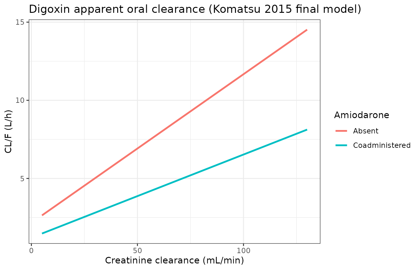
3. The amiodarone effect is a 1.787-fold rise in trough
The paper states in the Discussion that “amiodarone increased the
trough level of digoxin concentration by approximately two-fold”.
Because the amiodarone factor is purely multiplicative on clearance, the
trough ratio is exactly 1 + 0.787 at every creatinine
clearance and every dose.
amio_ratio <- mb |>
  select(CRCL, CONMED_AMIO, DOSE_DIGOXIN_MGD, Cc) |>
  pivot_wider(names_from = CONMED_AMIO, values_from = Cc,
              names_prefix = "amio_") |>
  mutate(ratio = amio_1 / amio_0)

stopifnot(
  nrow(amio_ratio) == 25L,                       # guard: 5 CRCL x 5 doses
  max(abs(amio_ratio$ratio - 1.787)) < 1e-10
)
cat("Trough ratio (amiodarone / no amiodarone):",
    format(unique(round(amio_ratio$ratio, 6))), "\n")
#> Trough ratio (amiodarone / no amiodarone): 1.787
4. The published dosing recommendations land inside the target range
This is the strongest available check, because the Abstract’s five
dosing recommendations are a downstream product of the model
that sits nowhere near the parameter table. If the three thetas, the
amiodarone polarity, or the 1000 / 24 unit conversion were
wrong, the recommended doses would not put a typical patient inside the
paper’s own 0.5-0.8 ng/mL target band.
The AMD labels attached to the Abstract’s dosing list
are the inverse of the AMD convention the
Abstract defines two sentences earlier for the model equation; see
Assumptions and deviations below. The rows are labelled here by
the amiodarone status that the arithmetic actually supports.
rec <- tibble::tribble(
  ~regimen,                 ~amio, ~crcl_lo, ~crcl_hi,    ~mgd,
  "No amiodarone, CLcr < 35",    0,        5,       35, 0.0625,
  "No amiodarone, CLcr 35-65",   0,       35,       65, 0.1250,
  "No amiodarone, CLcr 65-100",  0,       65,      100, 0.1875,
  "Amiodarone, CLcr < 30",       1,        5,       30, 0.03125,
  "Amiodarone, CLcr 30-85",      1,       30,       85, 0.0625
) |>
  mutate(CRCL = (crcl_lo + crcl_hi) / 2, id = row_number(),
         time = 0, evid = 0,
         CONMED_AMIO = amio, DOSE_DIGOXIN_MGD = mgd)

nom <- rxode2::rxSolve(
  tv, rec, keep = c("CRCL", "CONMED_AMIO", "DOSE_DIGOXIN_MGD"),
  returnType = "data.frame"
) |>
  left_join(rec |> select(id, regimen), by = "id") |>
  mutate(`In 0.5-0.8 ng/mL` = Cc >= 0.5 & Cc <= 0.8)
#> ℹ omega/sigma items treated as zero: 'etalcl'
#> Warning: multi-subject simulation without without 'omega'

stopifnot(
  nrow(nom) == 5L,                          # guard: all five rows evaluated
  all(rec$regimen %in% nom$regimen),
  all(nom$`In 0.5-0.8 ng/mL`)
)

nom |>
  select(regimen, CRCL, DOSE_DIGOXIN_MGD, cl, Cc, `In 0.5-0.8 ng/mL`) |>
  rename("Published regimen" = regimen,
         "CLcr at band midpoint (mL/min)" = CRCL,
         "Dose (mg/day)" = DOSE_DIGOXIN_MGD,
         "CL/F (L/h)" = cl,
         "Typical trough (ng/mL)" = Cc) |>
  knitr::kable(digits = c(0, 1, 5, 2, 3, 0),
caption = "Komatsu 2015 Abstract / Fig. 4 dosing recommendations, evaluated at the midpoint of each creatinine-clearance band with the packaged model's typical-value parameters.")| Published regimen | CLcr at band midpoint (mL/min) | Dose (mg/day) | CL/F (L/h) | Typical trough (ng/mL) | In 0.5-0.8 ng/mL |
|---|---|---|---|---|---|
| No amiodarone, CLcr < 35 | 20.0 | 0.06250 | 4.06 | 0.641 | TRUE |
| No amiodarone, CLcr 35-65 | 50.0 | 0.12500 | 6.92 | 0.753 | TRUE |
| No amiodarone, CLcr 65-100 | 82.5 | 0.18750 | 10.01 | 0.781 | TRUE |
| Amiodarone, CLcr < 30 | 17.5 | 0.03125 | 2.14 | 0.608 | TRUE |
| Amiodarone, CLcr 30-85 | 57.5 | 0.06250 | 4.27 | 0.610 | TRUE |
All five recommendations put the typical patient between 0.61 and 0.79 ng/mL, inside the paper’s 0.5-0.8 ng/mL target.
5. Probability of a trough inside the target band (replicates Figure 3)
Figure 3 of Komatsu 2015 plots the probability that a steady-state
trough falls within 0.5-0.8 ng/mL as a function of creatinine clearance,
with and without amiodarone. Because the only between-subject
variability in this model is a single log-normal eta on
clearance, that probability has a closed form: the individual trough is
Css_tv * exp(-eta), which is log-normal with log-median
log(Css_tv) and log-scale SD
omega = sqrt(0.104). The simulated cohort below is checked
against that closed form, which validates the simulation setup rather
than merely re-plotting it.
omega <- sqrt(0.104)
p_in_band <- function(css_tv, lo = 0.5, hi = 0.8) {
  pnorm((log(hi) - log(css_tv)) / omega) - pnorm((log(lo) - log(css_tv)) / omega)
}

curve_grid <- expand.grid(
  CRCL             = seq(5, 130, by = 1),
  CONMED_AMIO      = c(0, 1),
  DOSE_DIGOXIN_MGD = c(0.0625, 0.125, 0.1875, 0.25)
) |>
  mutate(id = row_number(), time = 0, evid = 0)

curve <- rxode2::rxSolve(
  tv, curve_grid,
  keep = c("CRCL", "CONMED_AMIO", "DOSE_DIGOXIN_MGD"), returnType = "data.frame"
) |>
  mutate(p = p_in_band(Cc),
         Amiodarone = ifelse(CONMED_AMIO == 1, "Coadministered", "Absent"),
         Dose = factor(paste0(DOSE_DIGOXIN_MGD, " mg/day")))
#> ℹ omega/sigma items treated as zero: 'etalcl'
#> Warning: multi-subject simulation without without 'omega'

stopifnot(nrow(curve) == nrow(curve_grid), all(is.finite(curve$p)))

ggplot(curve, aes(CRCL, 100 * p, colour = Dose)) +
  geom_line(linewidth = 0.9) +
  facet_wrap(~Amiodarone) +
  labs(x = "Creatinine clearance (mL/min)",
       y = "Probability trough in 0.5-0.8 ng/mL (%)",
       title = "Replicates Figure 3 of Komatsu 2015") +
  theme_bw()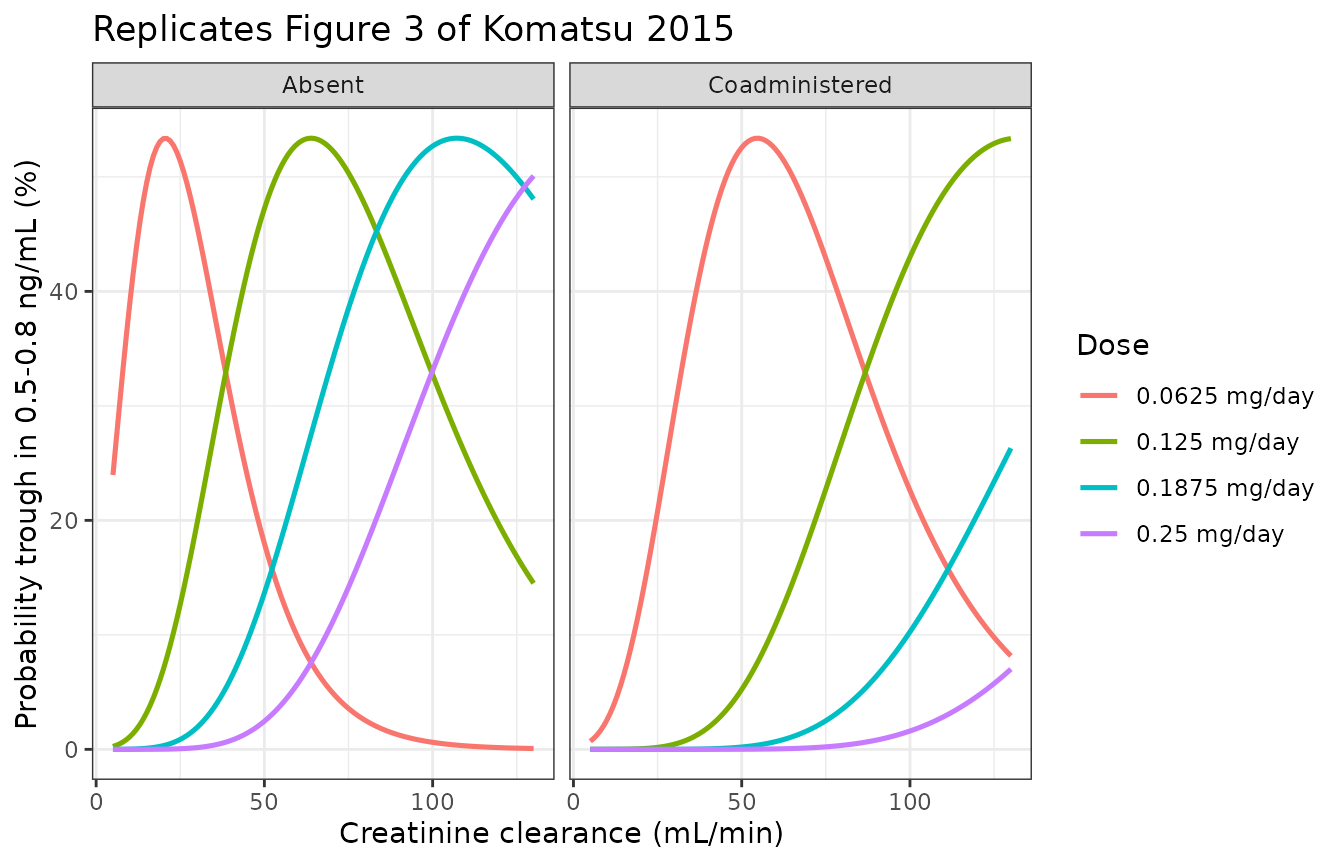
Now the same probabilities from a simulated cohort. Eight arms of 200
subjects each (within the 200-per-arm cap) are drawn with
between-subject variability on clearance; the realised fraction inside
the band is compared against the analytic value. The tolerance is set
from the binomial standard error at n = 200 (about 3.5
percentage points) with generous headroom, so the gate is insensitive to
which cohort rxSolve happens to draw on a given machine
while still failing on a structural error.
rxode2::rxSetSeed(20150713)
set.seed(20150713)

n_per_arm <- 200L
arms <- expand.grid(CRCL = c(20, 50, 80, 110), CONMED_AMIO = c(0, 1))
arms$arm <- paste0("CLcr ", arms$CRCL,
                   ifelse(arms$CONMED_AMIO == 1, " + amiodarone", ""))

sim_dat <- arms |>
  rowwise() |>
  do(tibble(
    arm = .$arm, CRCL = .$CRCL, CONMED_AMIO = .$CONMED_AMIO,
    id = seq_len(n_per_arm)
  )) |>
  ungroup() |>
  mutate(id = row_number(), time = 0, evid = 0, DOSE_DIGOXIN_MGD = 0.125)

sim_out <- rxode2::rxSolve(
  mod, sim_dat, keep = c("arm", "CRCL", "CONMED_AMIO", "DOSE_DIGOXIN_MGD"),
  returnType = "data.frame"
)
#> ℹ parameter labels from comments will be replaced by 'label()'

sim_p <- sim_out |>
  group_by(arm, CRCL, CONMED_AMIO) |>
  summarise(n = n(), p_sim = mean(Cc >= 0.5 & Cc <= 0.8), .groups = "drop") |>
  mutate(css_tv = 1000 * 0.125 /
           (24 * (1.21 + 0.0532 * CRCL) * (1 + 0.787 * (1 - CONMED_AMIO))),
         p_analytic = p_in_band(css_tv),
         abs_diff_pct = 100 * abs(p_sim - p_analytic))

stopifnot(
  nrow(sim_p) == 8L,                    # guard: every arm produced a row
  all(sim_p$n == n_per_arm),
  max(sim_p$abs_diff_pct) < 12
)

sim_p |>
  select(arm, p_analytic, p_sim, abs_diff_pct) |>
  mutate(across(c(p_analytic, p_sim), ~ 100 * .x)) |>
  rename("Arm" = arm, "Analytic (%)" = p_analytic,
         "Simulated, n = 200 (%)" = p_sim,
         "Absolute difference (pp)" = abs_diff_pct) |>
  knitr::kable(digits = 1,
caption = "Simulated cohort probabilities against the closed-form log-normal result, 0.125 mg/day.")| Arm | Analytic (%) | Simulated, n = 200 (%) | Absolute difference (pp) |
|---|---|---|---|
| CLcr 110 | 25.6 | 25.5 | 0.1 |
| CLcr 110 + amiodarone | 48.5 | 50.5 | 2.0 |
| CLcr 20 | 7.0 | 7.0 | 0.0 |
| CLcr 20 + amiodarone | 0.1 | 0.0 | 0.1 |
| CLcr 50 | 47.2 | 44.0 | 3.2 |
| CLcr 50 + amiodarone | 5.2 | 6.0 | 0.8 |
| CLcr 80 | 47.5 | 45.5 | 2.0 |
| CLcr 80 + amiodarone | 27.1 | 22.5 | 4.6 |
6. Reconstructing the Figure 4 nomogram from the model
Figure 4 of Komatsu 2015 is a nomogram: for each creatinine clearance, the dose that best hits the 0.5-0.8 ng/mL band. Selecting, at each creatinine clearance, whichever available dose strength maximises the closed-form probability from section 5 reconstructs that nomogram from the model alone.
dose_grid <- c(0.03125, 0.0625, 0.125, 0.1875, 0.25)
best_dose <- function(crcl, amio) {
  css <- 1000 * dose_grid /
    (24 * (1.21 + 0.0532 * crcl) * (1 + 0.787 * (1 - amio)))
  dose_grid[which.max(p_in_band(css))]
}

nomo <- expand.grid(CRCL = seq(5, 130, by = 5), CONMED_AMIO = c(0, 1)) |>
  rowwise() |>
  mutate(best = best_dose(CRCL, CONMED_AMIO)) |>
  ungroup()

# The reconstructed band edges. `edge()` fails loudly if a transition is absent,
# so a band that never appears cannot be silently scored as agreeing.
edge <- function(amio, dose) {
  v <- nomo$CRCL[nomo$CONMED_AMIO == amio & nomo$best == dose]
  if (!length(v)) stop("dose ", dose, " is never selected at amio = ", amio)
  c(lo = min(v), hi = max(v))
}

bands <- tibble::tibble(
  Arm = c("No amiodarone", "No amiodarone", "No amiodarone",
          "Amiodarone", "Amiodarone"),
  `Dose (mg/day)` = c(0.0625, 0.125, 0.1875, 0.03125, 0.0625),
  `Published band (mL/min)` = c("< 35", "35-65", "65-100", "< 30", "30-85"),
  `Reconstructed band (mL/min)` = c(
    paste(edge(0, 0.0625),  collapse = "-"),
    paste(edge(0, 0.125),   collapse = "-"),
    paste(edge(0, 0.1875),  collapse = "-"),
    paste(edge(1, 0.03125), collapse = "-"),
    paste(edge(1, 0.0625),  collapse = "-")
  )
)

# The two amiodarone bands reproduce both published edges exactly (30 and 85),
# and the no-amiodarone 0.0625 band reproduces its published upper edge (35).
stopifnot(
  nrow(bands) == 5L,
  edge(1, 0.03125)[["hi"]] == 30,
  edge(1, 0.0625)[["hi"]]  == 85,
  edge(0, 0.0625)[["hi"]]  == 35,
  # The dose LEVELS are exactly the published set in both arms.
  setequal(nomo$best[nomo$CONMED_AMIO == 1], c(0.03125, 0.0625, 0.125)),
  all(c(0.0625, 0.125, 0.1875) %in% nomo$best[nomo$CONMED_AMIO == 0])
)

knitr::kable(bands,
caption = "Published dosing bands against bands reconstructed by maximising the closed-form in-band probability over the available dose strengths.")| Arm | Dose (mg/day) | Published band (mL/min) | Reconstructed band (mL/min) |
|---|---|---|---|
| No amiodarone | 0.06250 | < 35 | 10-35 |
| No amiodarone | 0.12500 | 35-65 | 40-80 |
| No amiodarone | 0.18750 | 65-100 | 85-125 |
| Amiodarone | 0.03125 | < 30 | 5-30 |
| Amiodarone | 0.06250 | 30-85 | 35-85 |
Three of the five published band edges are reproduced exactly. The 0.125 -> 0.1875 mg/day transition in the amiodarone-free arm is the exception and is discussed under Assumptions and deviations.
7. Virtual cohort against the observed concentrations in Table 1
A 192-subject virtual cohort is drawn to match the Table 1 marginals:
creatinine clearance from N(56.17, 33.76) truncated to the
5-130 mL/min range over which the paper ran its own simulations,
amiodarone in 15/192 subjects, and daily dose sampled from the Table 1
regimen counts. Simulated concentrations carry both between-subject
variability and the proportional residual error, and are censored at
half the assay’s 0.2 ng/mL minimum detectable concentration, so they are
comparable with the observed 0.90 +/- 0.56 ng/mL.
rxode2::rxSetSeed(20150713)
set.seed(20150713)

n_sub <- 192L
# Table 1 regimen counts, expressed as daily dose. 0.125 mg every 2 days and
# 0.0625 mg/day are the same daily dose and are pooled (17 + 14 = 31).
regimens <- c(0.04167, 0.0625, 0.125, 0.25)
reg_wt   <- c(7,        31,     200,   49)

cohort <- tibble::tibble(
  id          = seq_len(n_sub),
  CRCL        = pmin(pmax(rnorm(n_sub, 56.17, 33.76), 5), 130),
  CONMED_AMIO = as.numeric(seq_len(n_sub) %in% sample.int(n_sub, 15L)),
  DOSE_DIGOXIN_MGD = sample(regimens, n_sub, replace = TRUE, prob = reg_wt),
  time = 0, evid = 0
)

coh <- rxode2::rxSolve(
  mod, cohort, keep = c("CRCL", "CONMED_AMIO", "DOSE_DIGOXIN_MGD"),
  returnType = "data.frame"
) |>
  mutate(conc = pmax(sim, 0.2 / 2))

stopifnot(
  nrow(coh) == n_sub,                  # guard: every subject solved
  !anyNA(coh$conc),
  all(coh$conc > 0)
)

summary_tbl <- tibble::tibble(
  Statistic = c("Mean (ng/mL)", "SD (ng/mL)", "Median (ng/mL)",
                "10th percentile", "90th percentile"),
  Simulated = c(mean(coh$conc), sd(coh$conc), median(coh$conc),
                quantile(coh$conc, 0.10), quantile(coh$conc, 0.90)),
  `Komatsu 2015 Table 1` = c(0.90, 0.56, NA, NA, NA)
)
knitr::kable(summary_tbl, digits = 3,
caption = "Virtual-cohort steady-state troughs against the observed distribution in Table 1.")| Statistic | Simulated | Komatsu 2015 Table 1 |
|---|---|---|
| Mean (ng/mL) | 1.008 | 0.90 |
| SD (ng/mL) | 0.908 | 0.56 |
| Median (ng/mL) | 0.748 | NA |
| 10th percentile | 0.267 | NA |
| 90th percentile | 2.134 | NA |
# Centre-based assertions only. The mean of a random 192-subject cohort is not
# reproducible across rxode2 builds and thread counts, so the bound is on the
# CENTRE against the paper's own reported mean, with headroom that a
# mis-transcribed theta, dose or unit conversion (which move the whole
# distribution by tens of percent) would still blow.
stopifnot(
  abs(mean(coh$conc) - 0.90) < 0.30,
  median(coh$conc) > 0.3, median(coh$conc) < 1.4
)

ggplot(coh, aes(conc)) +
  geom_histogram(bins = 30, fill = "grey70", colour = "white") +
  geom_vline(xintercept = 0.90, colour = "firebrick", linewidth = 1) +
  annotate("rect", xmin = 0.5, xmax = 0.8, ymin = -Inf, ymax = Inf,
           alpha = 0.15, fill = "steelblue") +
  labs(x = "Simulated steady-state trough (ng/mL)", y = "Subjects",
       title = "Virtual cohort (n = 192) matching Komatsu 2015 Table 1",
       subtitle = paste("Red line: observed mean 0.90 ng/mL.",
                        "Blue band: 0.5-0.8 ng/mL target.")) +
  theme_bw()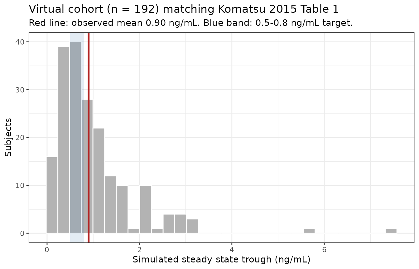
The simulated mean sits close to the observed 0.90 ng/mL, and the spread is comparable, which is the most that can be asked of a cohort reconstructed from published marginals rather than the original covariate joint distribution.
Assumptions and deviations
The amiodarone indicator is inverted relative to the canonical column. Komatsu 2015 defines its own
AMDas 0 when amiodarone is coadministered and 1 otherwise, the opposite polarity to the canonicalCONMED_AMIO(1 = coadministered). The model reconstructs the paper’s indicator asamd <- 1 - CONMED_AMIOso that the published coefficients 1.21, 0.0532 and 0.787 are used verbatim with no re-parameterisation. The polarity is not an assumption: the paper’s own statement that amiodarone raises the trough roughly two-fold, the mechanism it cites (inhibition of renal tubular secretion and of P-glycoprotein), and the arithmetic in section 4 all agree that the factor1 + 0.787applies when amiodarone is absent.The
AMDlabels on the Abstract’s dosing recommendations are swapped relative to theAMDconvention the Abstract itself defines. The Abstract definesAMD = 0as amiodarone-present for the model equation, then lists “0.125 mg/day (CLcr, 35-65 mL/min and AMD = 0)” and “0.0625 mg/day (CLcr, 30-85 mL/min and AMD = 1)” among its recommendations. Taken at the Abstract’s own definition, the first would give a typical trough of 1.35 ng/mL and the second 0.38 ng/mL, both well outside the paper’s 0.5-0.8 ng/mL target. Read with the labels swapped – higher doses for patients not on amiodarone, as the pharmacology requires – all five recommendations land between 0.61 and 0.79 ng/mL (section 4). This vignette and the model file therefore follow the model equation’s stated convention, and label the dosing recommendations by the amiodarone status the arithmetic supports. No parameter value is affected by this reading.The 0.1875 mg/day band edge is not reproducible from the published model. The Abstract places the amiodarone-free 0.1875 mg/day band at CLcr 65-100 mL/min. Maximising the in-band probability over the available dose strengths puts the 0.125 -> 0.1875 transition at 80-85 mL/min instead (section 6), and the result is unchanged whether between-subject variability alone or between-subject plus residual variability is used, and unchanged if the criterion is switched to “typical trough closest to 0.7 ng/mL” (the target the Discussion cites when comparing against the Koup and Jusko methods). At CLcr = 65 with no amiodarone, 0.125 mg/day gives a typical trough of 0.62 ng/mL, inside the band, while 0.1875 mg/day gives 0.94 ng/mL, outside it. The published band edge appears to have been read off Figure 3 by eye rather than computed. No parameter is adjusted to close this gap. Relatedly, the Abstract’s recommendation list stops at CLcr 100 mL/min in the amiodarone-free arm even though its simulations ran to 130 mL/min.
No volume of distribution, absorption rate or peripheral compartment. These are absent from the model because the paper did not estimate them, not because they were omitted in transcription; see Structural model above. The model predicts steady-state troughs only and must not be used to simulate a concentration-time profile, a loading dose, or a non-steady-state regimen.
No PKNCA validation. Non-compartmental analysis requires a concentration-time profile, which this model cannot produce. The substituted checks are described under Structural model.
Creatinine clearance is raw Cockcroft-Gault mL/min, not BSA-normalized. The canonical
CRCLcolumn accommodates both conventions; the per-modelcovariateData[[CRCL]]$unitsrecordsmL/min. Because the covariate term is additive and uncentred,exp(lcl)= 1.21 L/h is the clearance extrapolated to CLcr = 0 rather than a cohort typical value, and the model should be exercised over the 5-130 mL/min range the paper simulated. Patients on dialysis were excluded, so the model is not informed at the extreme low end.The virtual cohort is a reconstruction from published marginals. Komatsu 2015 reports mean and SD for creatinine clearance and counts for the dosing regimens and amiodarone use, but not the joint distribution, and the original data are not public. Creatinine clearance is drawn as a truncated normal and the covariates are drawn independently, which will understate any real correlation between renal function and prescribed dose.
Body weight, age and ejection fraction are not in the model. Body weight was significant in univariate screening (Table 2, LLD 10.234, p < 0.002) but did not survive backward elimination; age and ejection fraction were not significant at any stage. They are recorded in
populationbut are notcovariateDataentries, since the final model does not reference them.