The model
Jia_2025_tak_071 implements the final population
pharmacokinetic model for TAK-071 published by Jia et al. (2025),
Clinical Pharmacology in Drug Development 14(11):856-868, doi:10.1002/cpdd.1579.
TAK-071 is a muscarinic M1 positive allosteric modulator investigated for cognitive impairment and falls associated with Parkinson disease. It behaves as a Biopharmaceutics Classification System Class II compound (poorly soluble, highly permeable), which produces a complex oral absorption profile that the authors described with a lag time, a short transit chain, and two parallel first-order absorption routes feeding a single disposition compartment.
The structural equations below come from the NONMEM control stream of the final model, reproduced verbatim in the paper’s Supplemental Code (Supplemental Information pages S15-S17). Parameter values come from Table 1.
mod <- rxode2::rxode2(readModelDb("Jia_2025_tak_071"))
#> ℹ parameter labels from comments will be replaced by 'label()'
#> Warning: some etas defaulted to non-mu referenced, possible parsing error: etalogitfslow, etalka_slow
#> as a work-around try putting the mu-referenced expression on a simple line
mod
#>  ── rxode2-based free-form 6-cmt ODE model ──────────────────────────────────────
#>  ── Initalization: ──
#> Fixed Effects ($theta):
#>                 ltlag                  lmtt            logitfslow
#>            -1.6094379             0.2926696             1.4114846
#>              lka_slow             lka_quick                   lcl
#>            -0.1244301             4.1382498            -0.5691612
#>                   lvc               lfdepot        e_dose_ka_slow
#>             3.8607297             0.0000000            -0.8850000
#> e_form_tablet_ka_slow   e_form_tablet_fslow              e_age_cl
#>             3.2958369             0.4190000            -0.1710000
#>               e_wt_vc         e_dose_fdepot       propSdIntensive
#>             0.9130000            -0.0965000             0.1150000
#>          propSdSparse        addSdIntensive           addSdSparse
#>             0.1391500             5.2900000             6.4009000
#>
#> Omega ($omega):
#>               etalmtt etalogitfslow etalka_slow   etalcl   etalvc
#> etalmtt        0.3969        0.0000    0.000000 0.000000 0.000000
#> etalogitfslow  0.0000        1.2769    0.000000 0.000000 0.000000
#> etalka_slow    0.0000        0.0000    0.620944 0.000000 0.000000
#> etalcl         0.0000        0.0000    0.000000 0.139129 0.000000
#> etalvc         0.0000        0.0000    0.000000 0.000000 0.054289
#> attr(,"lotriLabels")
#> [1] "Table 1 MTT BSV 0.630 (RSE 2.8%, 95% CI 0.596-0.665) -> 69.8% CV"
#> [2] "Table 1 Fraction absorbed slowly BSV 1.13 (RSE 3.8%, 95% CI 1.05-1.21), additive on the logit scale"
#> [3] "Table 1 Absorption rate BSV 0.788 (RSE 4.0%, 95% CI 0.727-0.849)"
#> [4] "Table 1 Clearance BSV 0.373 (RSE 3.2%, 95% CI 0.349-0.396) -> 38.6% CV"
#> [5] "Table 1 Volume BSV 0.233 (RSE 2.6%, 95% CI 0.221-0.245) -> 23.6% CV"
#> attr(,"lotriFix")
#>               etalmtt etalogitfslow etalka_slow etalcl etalvc
#> etalmtt         FALSE         FALSE       FALSE  FALSE  FALSE
#> etalogitfslow   FALSE         FALSE       FALSE  FALSE  FALSE
#> etalka_slow     FALSE         FALSE       FALSE  FALSE  FALSE
#> etalcl          FALSE         FALSE       FALSE  FALSE  FALSE
#> etalvc          FALSE         FALSE       FALSE  FALSE  FALSE
#>
#> States ($state or $stateDf):
#>   Compartment Number Compartment Name
#> 1                  1            depot
#> 2                  2         transit1
#> 3                  3         transit2
#> 4                  4           depot2
#> 5                  5           depot3
#> 6                  6          central
#>  ── μ-referencing ($muRefTable): ──
#>   theta     eta level covariates
#> 1  lmtt etalmtt    id
#> 2   lcl  etalcl    id
#> 3   lvc  etalvc    id
#>
#>  ── Model (Normalized Syntax): ──
#> function() {
#>     compartmentData <- list(depot = list(analyte = "TAK-071",
#>         units = "mg", specimen = "administration site", verified = TRUE),
#>         transit1 = list(analyte = "TAK-071", units = "mg", specimen = "administration site",
#>             verified = TRUE), transit2 = list(analyte = "TAK-071",
#>             units = "mg", specimen = "administration site", verified = TRUE),
#>         depot2 = list(analyte = "TAK-071", units = "mg", specimen = "administration site",
#>             verified = TRUE), depot3 = list(analyte = "TAK-071",
#>             units = "mg", specimen = "administration site", verified = TRUE),
#>         central = list(analyte = "TAK-071", units = "mg", specimen = "plasma",
#>             verified = TRUE))
#>     covariateData <- list(AGE = list(description = "Baseline age",
#>         units = "years", type = "continuous", reference_category = NULL,
#>         notes = "Power covariate on clearance, normalized to 70 years (Methods, Population PK Model Development: 'age to 70 years'; Table 1 footnote c). Control-stream line TVCL = TVCL * (AGE/70)**THETA(17). Observed range 18-83 years (Table S1).",
#>         source_name = "AGE"), WT = list(description = "Baseline body weight",
#>         units = "kg", type = "continuous", reference_category = NULL,
#>         notes = "Power covariate on central volume, normalized to 80 kg (Methods, Population PK Model Development: 'body weight was normalized to 80 kg'; Table 1 footnote d). Control-stream line TVVC = TVVC * (WEIGHT/80)**THETA(16). Observed range 47.3-122 kg (Table S1).",
#>         source_name = "WEIGHT"), DOSE_TAK071_MG = list(description = "Administered TAK-071 dose level for the current dose record",
#>         units = "mg", type = "continuous", reference_category = NULL,
#>         notes = "Per-dose-record dose level in mg, normalized to 5 mg (Methods: 'dose to 5 mg'; Table 1 footnote b). Enters twice in the control stream: a power effect on relative bioavailability (TVFREL = THETA(1) * (DOSE/5)**THETA(14)) and a power effect on the slow absorption rate (TVKA = TVKA * (DOSE/5)**THETA(12)). Relative bioavailability and absorption rate both decrease as dose increases. Studied dose levels: 1, 3, 9, 20, 40, 80, 120, 160 mg single dose and 3, 5, 7.5, 9, 15 mg once daily.",
#>         source_name = "DOSE"), FORM_TABLET = list(description = "Oral formulation indicator: 1 = tablet, 0 = drug-in-capsule (DIC)",
#>         units = "(binary)", type = "binary", reference_category = "0 (drug-in-capsule, DIC)",
#>         notes = "Per-dose-record formulation flag. NOTE: the comparator here is a CAPSULE (drug-in-capsule), not the non-tablet oral liquid named as this canonical's default reference category -- same orientation as Wada_2023_sparsentan.R. Source column FORM, where FORM == 2 is the tablet; the control stream applies both tablet effects under IF(FORM == 2). The tablet carries (a) a multiplicative factor on the LOGIT of the slow-absorption fraction (IF(FORM == 2) TVFRAC_ = TVFRAC_ * THETA(15)) and (b) a multiplicative factor on the slow absorption rate (IF(FORM == 2) TVKA = TVKA * THETA(13)). Consistent with the observed median tmax of 2.00 h for the tablet vs 4.98 h for the capsule after a single 10 mg dose (Discussion).",
#>         source_name = "FORM"), SAMPLE_INTENSIVE = list(description = "Sampling-design indicator: 1 = dense (intensive) PK sampling, 0 = sparse PK sampling",
#>         units = "(binary)", type = "binary", reference_category = "0 (sparse sampling)",
#>         notes = "Source column SAMPLING, where SAMPLING == 2 is the sparse subset (participants with Parkinson disease in the Phase 2 main cohort, TAK-071-2002). Unlike the Macpherson 2015 founding example this flag does NOT vary within a subject in this analysis -- it is a per-subject design attribute, so set it once per participant. It switches three things in the control stream: the between-subject random effect on the logit slow-absorption fraction is suppressed (IF(SAMPLING == 2) FRAC_ = TVFRAC_), the between-subject random effect on the slow absorption rate is suppressed (IF(SAMPLING == 2) KA = TVKA), and the residual error is inflated (IF(SAMPLING == 2) W = W * THETA(11), ratio 1.21). Rationale (Results): 'The sparse PK data collected in patients with PD did not allow for reliable estimation of individual absorption rates and fraction parameters, which is why no random effects for ka and frac were estimated for this subset. In addition, the model could quantify an inflated residual variability in this subset of approximately 21%.'",
#>         source_name = "SAMPLING"))
#>     description <- "One-compartment population PK model for TAK-071 (muscarinic M1 positive allosteric modulator) in healthy adults and participants with Parkinson disease, with a fixed absorption lag, a 3-step transit chain, and parallel slow/quick first-order absorption; dose effects on relative bioavailability and absorption rate, formulation (tablet vs drug-in-capsule) effects on the slow-absorption fraction and rate, age on clearance, and body weight on central volume"
#>     population <- list(species = "human", n_subjects = 165L,
#>         n_studies = 2L, age_range = "18-83 years", age_median = "44 years",
#>         weight_range = "47.3-122 kg", weight_median = "78.7 kg",
#>         sex_female_pct = 11.8, race_ethnicity = c(White = 65.4,
#>             `Black or African American` = 15, Asian = 12.4, Multiple = 3.3,
#>             `Native Hawaiian or other Pacific Islander` = 2,
#>             `American Indian or Alaska Native` = 0.7, `Not reported` = 1.3),
#>         disease_state = "healthy adults, and participants with Parkinson disease with cognitive impairment and an elevated risk of falls",
#>         dose_range = "1-160 mg single oral dose and 3-15 mg once daily (Phase 1, TAK-071-1001); 7.5 mg single dose and 5 or 7.5 mg once daily (Phase 2, TAK-071-2002)",
#>         renal_function = "creatinine clearance 56.9-180 mL/min/1.73m2; eGFR 57.1-143 mL/min (Table S1); neither was a significant covariate on clearance",
#>         notes = "Two studies: TAK-071-1001 (Phase 1 single- and multiple-ascending-dose with a 3-way crossover food-effect and relative-bioavailability arm, healthy adults 18-55 years, 96% men, 16% Japanese, NCT02769065) and TAK-071-2002 (Phase 2 randomized double-blind placebo-controlled 2-period crossover, sentinel cohort of healthy participants older than 55 years plus a main cohort of participants with Parkinson disease aged 40-85 years, no Japanese participants, NCT04334317). Counts differ between the paper's own sources: the Abstract and the Results Data Set section give 165 participants (112 healthy = 104 from TAK-071-1001 plus 8 sentinel, and 53 with Parkinson disease = 37 at 5 mg plus 16 at 7.5 mg), whereas Table S1 reports 153 individuals (92 healthy, 61 with Parkinson disease). The demographic summaries recorded here (median/range, sex, race) are Table S1 values and are therefore computed on the n = 153 denominator.")
#>     reference <- "Jia H, Facius A, Jennings R, Hang Y, Padmanabhan J, Shanbhag NM, Harel BT, Simen A, Yin W. Population Pharmacokinetic and Exposure-Response Analysis of the Cognitive Effects of TAK-071 in Participants With Parkinson Disease and Cognitive Impairment. Clin Pharmacol Drug Dev. 2025;14(11):856-868. doi:10.1002/cpdd.1579. Structural equations from the Supplemental Code (NONMEM control stream of the final model, Supplemental Information page S15-S17); parameter values from Table 1."
#>     units <- list(time = "h", dosing = "mg", concentration = "ng/mL")
#>     vignette <- "Jia_2025_tak_071"
#>     ini({
#>         ltlag <- fix(-1.6094379124341)
#>         label("Absorption lag time (log h)")
#>         lmtt <- 0.29266961396282
#>         label("Mean transit time, excluding the lag (log h)")
#>         logitfslow <- 1.41148460994845
#>         label("Fraction absorbed by the slow route (logit)")
#>         lka_slow <- -0.124430078378177
#>         label("Slow first-order absorption rate at 5 mg, drug-in-capsule (log 1/h)")
#>         lka_quick <- 4.13824979866314
#>         label("Quick first-order absorption rate at 5 mg, drug-in-capsule (log 1/h)")
#>         lcl <- -0.569161200778954
#>         label("Clearance at 70 years of age (log L/h)")
#>         lvc <- 3.8607297110406
#>         label("Central volume of distribution at 80 kg (log L)")
#>         lfdepot <- fix(0)
#>         label("Relative bioavailability at the 5 mg reference dose (log fraction)")
#>         e_dose_ka_slow <- -0.885
#>         label("Power exponent on (DOSE/5) for the slow absorption rate (unitless)")
#>         e_form_tablet_ka_slow <- 3.29583686600433
#>         label("Log ratio of tablet to drug-in-capsule slow absorption rate (unitless)")
#>         e_form_tablet_fslow <- 0.419
#>         label("Ratio applied to the logit slow-absorption fraction for tablets (unitless)")
#>         e_age_cl <- -0.171
#>         label("Power exponent on (AGE/70) for clearance (unitless)")
#>         e_wt_vc <- 0.913
#>         label("Power exponent on (WT/80) for central volume (unitless)")
#>         e_dose_fdepot <- -0.0965
#>         label("Power exponent on (DOSE/5) for relative bioavailability (unitless)")
#>         propSdIntensive <- 0.115
#>         label("Proportional residual error, dense sampling (fraction)")
#>         propSdSparse <- 0.13915
#>         label("Proportional residual error, sparse sampling (fraction)")
#>         addSdIntensive <- 5.29
#>         label("Additive residual error, dense sampling (ng/mL)")
#>         addSdSparse <- 6.4009
#>         label("Additive residual error, sparse sampling (ng/mL)")
#>         etalmtt ~ 0.3969
#>         label("Table 1 MTT BSV 0.630 (RSE 2.8%, 95% CI 0.596-0.665) -> 69.8% CV")
#>         etalogitfslow ~ 1.2769
#>         label("Table 1 Fraction absorbed slowly BSV 1.13 (RSE 3.8%, 95% CI 1.05-1.21), additive on the logit scale")
#>         etalka_slow ~ 0.620944
#>         label("Table 1 Absorption rate BSV 0.788 (RSE 4.0%, 95% CI 0.727-0.849)")
#>         etalcl ~ 0.139129
#>         label("Table 1 Clearance BSV 0.373 (RSE 3.2%, 95% CI 0.349-0.396) -> 38.6% CV")
#>         etalvc ~ 0.054289
#>         label("Table 1 Volume BSV 0.233 (RSE 2.6%, 95% CI 0.221-0.245) -> 23.6% CV")
#>     })
#>     model({
#>         tlag <- exp(ltlag)
#>         mtt <- exp(lmtt + etalmtt)
#>         ktr <- 4/mtt
#>         logitfslowTv <- logitfslow * ((1 - FORM_TABLET) + e_form_tablet_fslow *
#>             FORM_TABLET)
#>         fslow <- expit(logitfslowTv + etalogitfslow * SAMPLE_INTENSIVE,
#>             0, 1)
#>         kaCov <- e_dose_ka_slow * log(DOSE_TAK071_MG/5) + e_form_tablet_ka_slow *
#>             FORM_TABLET + etalka_slow * SAMPLE_INTENSIVE
#>         ka_slow <- exp(lka_slow + kaCov)
#>         ka_quick <- exp(lka_quick + kaCov)
#>         cl <- exp(lcl + etalcl) * (AGE/70)^e_age_cl
#>         vc <- exp(lvc + etalvc) * (WT/80)^e_wt_vc
#>         kel <- cl/vc
#>         d/dt(depot) <- -ktr * depot
#>         d/dt(transit1) <- ktr * depot - ktr * transit1
#>         d/dt(transit2) <- ktr * transit1 - ktr * transit2
#>         d/dt(depot2) <- ktr * fslow * transit2 - ka_slow * depot2
#>         d/dt(depot3) <- ktr * (1 - fslow) * transit2 - ka_quick *
#>             depot3
#>         d/dt(central) <- ka_slow * depot2 + ka_quick * depot3 -
#>             kel * central
#>         alag(depot) <- tlag
#>         f(depot) <- exp(lfdepot) * (DOSE_TAK071_MG/5)^e_dose_fdepot
#>         Cc <- 1000 * central/vc
#>         propSd <- propSdIntensive * SAMPLE_INTENSIVE + propSdSparse *
#>             (1 - SAMPLE_INTENSIVE)
#>         addSd <- addSdIntensive * SAMPLE_INTENSIVE + addSdSparse *
#>             (1 - SAMPLE_INTENSIVE)
#>         Cc ~ prop(propSd) + add(addSd)
#>     })
#> }
Structure
The control stream uses ADVAN5 with six
compartments:
| Control stream | nlmixr2lib state | Role |
|---|---|---|
GUT (DEFDOSE) |
depot |
dosing compartment, carries the 0.2 h lag |
TR1 |
transit1 |
transit compartment |
TR2 |
transit2 |
transit compartment, splits the dose |
ABS1 |
depot2 |
slow absorption compartment |
ABS2 |
depot3 |
quick absorption compartment |
CENTRAL (DEFOBS) |
central |
plasma disposition |
Drug leaves TR2 at the transit rate ktr and
is split between the slow route (fraction fslow) and the
quick route (1 - fslow); the two absorption compartments
then empty into central at ka_slow and
ka_quick. Elimination is first order.
Three details are load-bearing and are only resolvable from the control stream, not from Table 1 alone:
-
Table 1’s MTT of 1.54 h includes the fixed 0.2 h
lag. The control stream forms the transit rate from
TVMTT = THETA(3) - ALAG1, so the transit-chain mean transit time is 1.54 - 0.2 = 1.34 h andktr = (NT + 1) / MTT = 4 / 1.34withNT = 3. The Results text confirms it: “an MTT (including a fixed tlag of 0.2 hours), estimated at 1.54 hours”. -
The tablet effect on the slow-absorption fraction multiplies
the logit of the fraction, not the fraction itself. The control
stream line is
IF (FORM == 2) TVFRAC_ = TVFRAC_ * THETA(15)whereTVFRAC_ = logit(TVFRAC). Table 1 labels the 0.419 estimate only as a “ratio”, which invites the wrong reading. The tablet slow-absorbed fraction is thereforeexpit(logit(0.804) * 0.419) = 64.4%, not0.804 * 0.419 = 33.7%. -
The quick absorption rate is estimated as a ratio to the
slow rate (
KAQ = THETA(6),K5T6 = KA * KAQ), so it inherits the dose effect, the tablet effect and the single between-subject random effect that act on the slow rate.lka_quickis therefore set tolog(0.883 * 71.0), which equals the 62.7 1/h quoted in the Results text, and the same covariate/eta term is added to both rates inmodel().
Source trace
Every value in ini() traces to Table 1 unless noted.
Structural equations trace to the Supplemental Code.
| Model quantity | Value | Source |
|---|---|---|
ltlag |
log(0.2), fixed |
Supplemental Code $THETA(2) 0.2 FIX;
Results text |
lmtt |
log(1.54 - 0.2) |
Table 1 MTT TV 1.54 h; Supplemental Code
TVMTT = THETA(3) - ALAG1
|
logitfslow |
logit(0.804) |
Table 1 Fraction absorbed slowly TV 80.4% |
lka_slow |
log(0.883) |
Table 1 Absorption rate TV 0.883 1/h (footnote b: 5 mg, DIC) |
lka_quick |
log(0.883 * 71.0) |
Table 1 Absorption ratio quick/slow 71.0; Results text ka,quick = 62.7 |
lcl |
log(0.566) |
Table 1 Clearance TV 0.566 L/h (footnote c: age 70 y) |
lvc |
log(47.5) |
Table 1 Volume TV 47.5 L (footnote d: 80 kg) |
lfdepot |
log(1), fixed |
Supplemental Code $THETA(1) 100 FIX;
F1 = FREL/100
|
e_dose_ka_slow |
-0.885 | Table 1 Absorption rate dose-effect (power) |
e_form_tablet_ka_slow |
log(27.0) |
Table 1 Absorption rate tablet-effect (ratio) |
e_form_tablet_fslow |
0.419 | Table 1 Fraction tablet-effect (ratio, on the logit) |
e_age_cl |
-0.171 | Table 1 Clearance age-effect (power) |
e_wt_vc |
0.913 | Table 1 Volume body weight-effect (power) |
e_dose_fdepot |
-0.0965 | Table 1 Relative bioavailability dose-effect (power) |
| BSV (5 etas) | 0.630, 1.13, 0.788, 0.373, 0.233 | Table 1 BSV rows; footnote a states these are standard deviations |
| Residual error | 11.5%, 5.29 ng/mL, sparse ratio 1.21 | Table 1 RUV rows |
| Covariate reference values | 80 kg, 70 y, 5 mg | Methods, Population PK Model Development |
| ODE transfer rates | K1T2 ... K6T0 |
Supplemental Code $PK
|
| Concentration scaling | S6 = VC/1000 |
Supplemental Code $PK
|
Table 1’s random-effect rows are omega standard
deviations (footnote a). Squaring them and applying
Supplemental Equation 2, CV = sqrt(exp(omega^2) - 1),
reproduces the CV% values quoted in the Results text exactly: 0.630
gives 69.8% for MTT, 0.373 gives 38.6% for clearance and 0.233 gives
23.6% for central volume.
Population
The analysis pooled two studies:
- TAK-071-1001 (NCT02769065): Phase 1 single- and multiple-ascending-dose study in healthy adults aged 18-55 years, with a 3-way crossover food-effect and relative-bioavailability arm. Single doses 1-160 mg, multiple doses 3-15 mg once daily. 96% men; 16% Japanese participants.
- TAK-071-2002 (NCT04334317): Phase 2 randomized, double-blind, placebo-controlled, 2-period crossover study. A sentinel cohort of healthy participants older than 55 years received a single 7.5 mg dose; the main cohort of participants with Parkinson disease aged 40-85 years with cognitive impairment and elevated fall risk received 5 mg once daily (aged 66-85) or 7.5 mg once daily (aged 40-65) for 6 weeks per period.
pop <- readModelDb("Jia_2025_tak_071")()$population
#> Warning: some etas defaulted to non-mu referenced, possible parsing error: etalogitfslow, etalka_slow
#> as a work-around try putting the mu-referenced expression on a simple line
str(pop, max.level = 1)
#> List of 13
#>  $ species       : chr "human"
#>  $ n_subjects    : int 165
#>  $ n_studies     : int 2
#>  $ age_range     : chr "18-83 years"
#>  $ age_median    : chr "44 years"
#>  $ weight_range  : chr "47.3-122 kg"
#>  $ weight_median : chr "78.7 kg"
#>  $ sex_female_pct: num 11.8
#>  $ race_ethnicity: Named num [1:7] 65.4 15 12.4 3.3 2 0.7 1.3
#>   ..- attr(*, "names")= chr [1:7] "White" "Black or African American" "Asian" "Multiple" ...
#>  $ disease_state : chr "healthy adults, and participants with Parkinson disease with cognitive impairment and an elevated risk of falls"
#>  $ dose_range    : chr "1-160 mg single oral dose and 3-15 mg once daily (Phase 1, TAK-071-1001); 7.5 mg single dose and 5 or 7.5 mg on"| __truncated__
#>  $ renal_function: chr "creatinine clearance 56.9-180 mL/min/1.73m2; eGFR 57.1-143 mL/min (Table S1); neither was a significant covariate on clearance"
#>  $ notes         : chr "Two studies: TAK-071-1001 (Phase 1 single- and multiple-ascending-dose with a 3-way crossover food-effect and r"| __truncated__
Baseline characteristics (Table S1): median age 44 years (range 18-83), median body weight 78.7 kg (range 47.3-122), 11.8% women, 65.4% White, 15.0% Black or African American, 12.4% Asian.
Note that the paper reports two different participant counts: the Abstract and the Results Data Set section give 165 (112 healthy plus 53 with Parkinson disease), while Table S1 reports 153 (92 healthy, 61 with Parkinson disease). See “Assumptions and deviations” below.
Virtual cohorts
All cohorts below use tablets, matching the Phase 2 study. Body weights are drawn from a truncated normal distribution centred on the Table S1 median of 78.7 kg; the paper reports only the median and range, so the spread is an assumption. Ages are drawn uniformly across each cohort’s stated eligibility range.
set.seed(20250819)

make_cohort <- function(treatment, dose_mg, n, age_lo, age_hi, tablet,
                        intensive, obs_times, addl = 0, ii = 0, id_offset = 0) {
  ages <- runif(n, age_lo, age_hi)
  wts  <- pmax(45, pmin(125, rnorm(n, 78.7, 15)))
  ev <- rxode2::et(amt = dose_mg, ii = ii, addl = addl, cmt = "depot") |>
    rxode2::et(obs_times) |>
    rxode2::et(id = seq_len(n))
  d <- as.data.frame(ev)
  d$AGE <- ages[d$id]
  d$WT <- wts[d$id]
  d$DOSE_TAK071_MG <- dose_mg
  d$FORM_TABLET <- tablet
  d$SAMPLE_INTENSIVE <- intensive
  d$treatment <- treatment
  d$id <- d$id + id_offset
  d
}

# The quick absorption route has a very large rate constant (about 1250 1/h for
# a tablet at 7 mg), which makes the ODE system stiff enough that rxode2's
# default liblsoda solver fails for the occasional individual and silently
# returns NA. `method = "lsoda"` solves every individual; the helper asserts
# that no concentration came back missing so a solver failure can never pass
# silently into a summary.
solve_cohort <- function(events, seed, ...) {
  set.seed(seed)
  s <- rxode2::rxSolve(mod, events, method = "lsoda",
                       returnType = "data.frame", ...)
  stopifnot(!anyNA(s$Cc))
  s
}
Single-dose cohorts
The sentinel cohort reproduces the Phase 2 design exactly, including its published blood-sampling schedule (Supplemental Information, Sample Collection Time Points): pre-dose and 0.5, 1, 2, 3, 4, 6, 8, 10, 12, 14, 24, 48, 72, 96 and 168 hours post dose.
sched_p2 <- c(0, 0.5, 1, 2, 3, 4, 6, 8, 10, 12, 14, 24, 48, 72, 96, 168)
sched_p1 <- c(0, 0.5, 1, 2, 3, 4, 6, 8, 10, 12, 16, 24, 32, 40, 48, 72, 96, 168)

ev_single <- bind_rows(
  make_cohort("Sentinel 7.5 mg tablet", 7.5, 200, 56, 74, 1, 1, sched_p2, id_offset = 0),
  make_cohort("10 mg tablet",          10.0, 200, 18, 55, 1, 1, sched_p1, id_offset = 1000),
  make_cohort("10 mg capsule",         10.0, 200, 18, 55, 0, 1, sched_p1, id_offset = 2000)
)

sim_single <- solve_cohort(ev_single, seed = 101, keep = "treatment")
stopifnot(is.character(sim_single$treatment))
stopifnot(length(unique(sim_single$id)) == 600)
sim_single |>
  group_by(treatment, time) |>
  summarise(med = median(Cc), lo = quantile(Cc, 0.05),
            hi = quantile(Cc, 0.95), .groups = "drop") |>
  ggplot(aes(time, med, colour = treatment, fill = treatment)) +
  geom_ribbon(aes(ymin = lo, ymax = hi), alpha = 0.15, colour = NA) +
  geom_line(linewidth = 0.8) +
  scale_x_continuous(limits = c(0, 72)) +
  labs(x = "Time (h)", y = "TAK-071 plasma concentration (ng/mL)",
       colour = NULL, fill = NULL) +
  theme_bw() +
  theme(legend.position = "top")
#> Warning: Removed 6 rows containing missing values or values outside the scale range
#> (`geom_ribbon()`).
#> Warning: Removed 6 rows containing missing values or values outside the scale range
#> (`geom_line()`).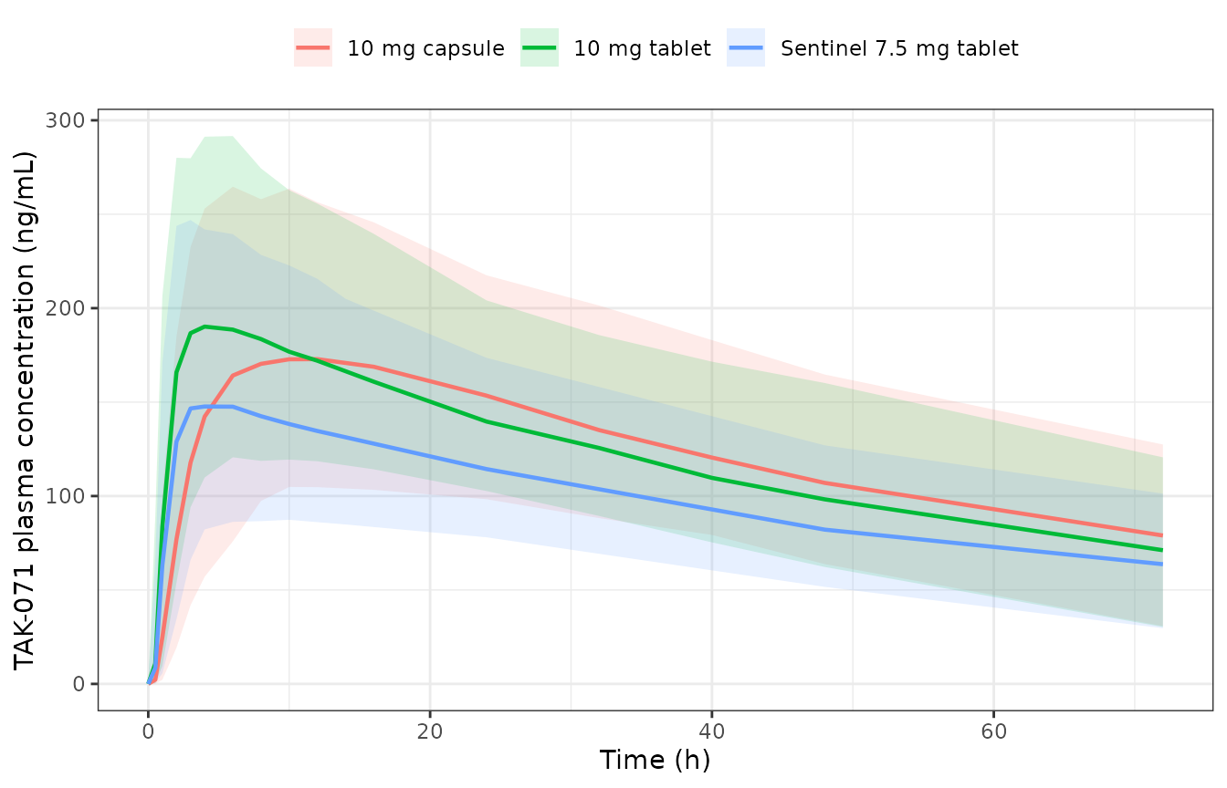
Simulated single-dose TAK-071 plasma profiles (median and 5th-95th percentiles of the individual predictions). The 10 mg capsule reaches its peak later than the 10 mg tablet, reproducing the formulation effect reported in the Discussion.
Multiple-dose cohorts (Parkinson disease main cohort)
The main cohort received 5 mg once daily (aged 66-85) or 7.5 mg once
daily (aged 40-65) for 6 weeks. Cohort sizes are scaled from the
published 37:16 split. These participants were sparsely sampled, so
SAMPLE_INTENSIVE = 0, which suppresses the between-subject
random effects on the absorption rate and the slow-absorption fraction
and inflates the residual error by the estimated 1.21 ratio, exactly as
the control stream does.
obs_md <- c(seq(0, 24, by = 0.5), seq(984, 1008, by = 0.5))

ev_md <- bind_rows(
  make_cohort("PD 5 mg QD",   5.0, 150, 66, 85, 1, 0, obs_md, addl = 41, ii = 24, id_offset = 0),
  make_cohort("PD 7.5 mg QD", 7.5,  65, 40, 65, 1, 0, obs_md, addl = 41, ii = 24, id_offset = 1000)
)

sim_md <- solve_cohort(ev_md, seed = 202, keep = "treatment")
stopifnot(length(unique(sim_md$id)) == 215)
Structural check: terminal half-life
The paper derives a secondary parameter, terminal half-life, as
ln(2) * Volume / Clearance, and reports “The
model-estimated terminal half-life was 58 hours”.
Replicating the published dose-selection simulation
This is the sharpest available check, because the paper reports the output of its own model simulation rather than an observed summary. From the Results:
Because nonclinical data suggested that the mean PK exposure should be kept below a Cmax,ss of 600 ng/mL and an AUCtau,ss of 14,000 ng x h/mL, the highest dose that can be administered to participants aged 40 and 85 years is 7 mg once daily, which provides the model-predicted geometric mean (80% prediction interval) Cmax,ss of 562 (374-863) ng/mL and AUCtau,ss of 11,900 (7410-19,200) ng x h/mL.
gm <- function(x) exp(mean(log(x)))
trap <- function(t, c) sum(diff(t) * (head(c, -1) + tail(c, -1)) / 2)

ev_7mg <- make_cohort("PD 7 mg QD", 7, 200, 70, 70, 1, 0,
                      seq(1008, 1032, by = 0.1), addl = 42, ii = 24)
sim_7mg <- solve_cohort(ev_7mg, seed = 303)

ss_7mg <- sim_7mg |>
  filter(time >= 1008) |>
  group_by(id) |>
  summarise(cmax = max(Cc), auctau = trap(time, Cc), .groups = "drop")

dose_sel <- tibble::tibble(
  Metric = c("Cmax,ss (ng/mL)", "AUCtau,ss (ng*h/mL)"),
  `Simulated geometric mean` = c(gm(ss_7mg$cmax), gm(ss_7mg$auctau)),
  `Simulated 80% PI` = c(
    sprintf("%.0f-%.0f", quantile(ss_7mg$cmax, 0.1), quantile(ss_7mg$cmax, 0.9)),
    sprintf("%.0f-%.0f", quantile(ss_7mg$auctau, 0.1), quantile(ss_7mg$auctau, 0.9))),
  `Published geometric mean` = c(562, 11900),
  `Published 80% PI` = c("374-863", "7410-19200")
) |>
  mutate(`Difference (%)` = 100 * (`Simulated geometric mean` /
                                     `Published geometric mean` - 1))

knitr::kable(dose_sel, digits = c(0, 0, 0, 0, 0, 1),
caption = "Replicates the 7 mg once-daily dose-selection simulation reported in the Results of Jia 2025.")| Metric | Simulated geometric mean | Simulated 80% PI | Published geometric mean | Published 80% PI | Difference (%) |
|---|---|---|---|---|---|
| Cmax,ss (ng/mL) | 555 | 354-920 | 562 | 374-863 | -1.2 |
| AUCtau,ss (ng*h/mL) | 11734 | 7082-20195 | 11900 | 7410-19200 | -1.4 |
Both metrics reproduce the published geometric means to within 2%, confirming that the relative-bioavailability dose effect, the clearance value and the absorption model are all encoded as the authors specified.
Age and body weight sensitivity
The paper concludes that neither age nor body weight warrants dose adjustment:
the difference in simulated TAK-071 PK exposure (Cmax,ss and AUCtau,ss) for people with PD aged 40 and 85 years, compared with the reference age of 70 years was less than 10%
and, for body weight (Figure S2),
The difference between the simulated PK exposure of TAK-071 in people with PD with a body weight of 120 and 50 kg and the reference body weight of 80 kg was within 10%
covariate_arm <- function(age, wt, n = 100, seed = 1) {
  ev <- rxode2::et(amt = 7, ii = 24, addl = 42, cmt = "depot") |>
    rxode2::et(seq(1008, 1032, by = 0.1)) |>
    rxode2::et(id = seq_len(n))
  d <- as.data.frame(ev)
  d$AGE <- age; d$WT <- wt
  d$DOSE_TAK071_MG <- 7; d$FORM_TABLET <- 1; d$SAMPLE_INTENSIVE <- 0
  s <- solve_cohort(d, seed = seed) |> filter(time >= 1008)
  s |> group_by(id) |>
    summarise(cmax = max(Cc), auctau = trap(time, Cc), .groups = "drop") |>
    summarise(cmax = gm(cmax), auctau = gm(auctau))
}

ref <- covariate_arm(70, 80, seed = 11)

sens <- bind_rows(
  bind_cols(tibble::tibble(Scenario = "Age 40 years (reference 70)"), covariate_arm(40, 80, seed = 12)),
  bind_cols(tibble::tibble(Scenario = "Age 85 years (reference 70)"), covariate_arm(85, 80, seed = 13)),
  bind_cols(tibble::tibble(Scenario = "Weight 50 kg (reference 80)"), covariate_arm(70, 50, seed = 14)),
  bind_cols(tibble::tibble(Scenario = "Weight 120 kg (reference 80)"), covariate_arm(70, 120, seed = 15))
) |>
  mutate(`Cmax,ss difference (%)` = 100 * (cmax / ref$cmax - 1),
         `AUCtau,ss difference (%)` = 100 * (auctau / ref$auctau - 1)) |>
  select(Scenario, `Cmax,ss difference (%)`, `AUCtau,ss difference (%)`)

knitr::kable(sens, digits = 1,
caption = "Age and body weight sensitivity of steady-state exposure at 7 mg once daily. Published claim: all differences below 10%.")| Scenario | Cmax,ss difference (%) | AUCtau,ss difference (%) |
|---|---|---|
| Age 40 years (reference 70) | -1.3 | -1.6 |
| Age 85 years (reference 70) | -0.8 | -0.6 |
| Weight 50 kg (reference 80) | 9.7 | 3.8 |
| Weight 120 kg (reference 80) | -3.8 | 0.7 |
stopifnot(all(abs(sens$`Cmax,ss difference (%)`) < 10))
stopifnot(all(abs(sens$`AUCtau,ss difference (%)`) < 10))
Every scenario stays inside the 10% band the paper reports, reproducing both no-dose-adjustment conclusions.
Noncompartmental analysis
Single dose
# Table 2 reports OBSERVED noncompartmental parameters, so the simulated
# analogue is `sim` (the model prediction plus residual error), not `Cc` (the
# noise-free individual prediction). This matters for Cmax in particular: an
# observed Cmax is the maximum of noisy samples and is therefore biased upward
# relative to the true peak. Concentrations are floored at zero because the
# additive residual error can push a simulated sample negative.
nca_conc <- sim_single |>
  filter(!is.na(sim)) |>
  transmute(id, time, treatment, Cc = pmax(sim, 0))

# Defensive time-zero row (extravascular dosing, so pre-dose Cc = 0).
nca_conc <- bind_rows(
  nca_conc,
  nca_conc |> distinct(id, treatment) |> mutate(time = 0, Cc = 0)
) |>
  distinct(id, treatment, time, .keep_all = TRUE) |>
  arrange(id, treatment, time)

nca_dose <- ev_single |>
  filter(evid == 1) |>
  select(id, time, amt, treatment)

conc_obj <- PKNCA::PKNCAconc(nca_conc, Cc ~ time | treatment + id,
                             concu = "ng/mL", timeu = "h")
dose_obj <- PKNCA::PKNCAdose(nca_dose, amt ~ time | treatment + id,
                             doseu = "mg")

intervals_single <- data.frame(
  start = 0, end = Inf,
  cmax = TRUE, tmax = TRUE, aucinf.obs = TRUE,
  half.life = TRUE, clast.obs = TRUE
)

nca_single <- PKNCA::pk.nca(
  PKNCA::PKNCAdata(conc_obj, dose_obj, intervals = intervals_single)
)
The paper reports observed noncompartmental parameters for the Phase 2 sentinel cohort (Table 2, n = 8, single 7.5 mg oral dose in healthy participants aged 56-74 years). Values are arithmetic means except tmax, which is a median.
published_single <- tibble::tribble(
  ~treatment,               ~cmax, ~tmax, ~aucinf.obs, ~half.life,
  "Sentinel 7.5 mg tablet",   195,  1.50,       15100,       70.7
)

cmp_single <- nlmixr2lib::ncaComparisonTable(
  simulated = nca_single,
  reference = published_single,
  by = "treatment",
  units = c(cmax = "ng/mL", tmax = "h", aucinf.obs = "ng*h/mL", half.life = "h"),
  tolerance_pct = 20
)

knitr::kable(
  cmp_single,
  digits = 1,
  caption = "Simulated vs. published noncompartmental parameters for the Phase 2 sentinel cohort (Jia 2025 Table 2). * marks rows differing from the published value by more than 20%."
)| NCA parameter | treatment | Reference | Simulated | % diff |
|---|---|---|---|---|
| Cmax (ng/mL) | Sentinel 7.5 mg tablet | 195 | 169 | -13.2% |
| Tmax (h) | Sentinel 7.5 mg tablet | 1.5 | 6 | +300.0%* |
| AUC0-∞ (obs) (ng*h/mL) | Sentinel 7.5 mg tablet | 15100 | 12500 | -17.5% |
| t½ (h) | Sentinel 7.5 mg tablet | 70.7 | 56.5 | -20.1%* |
Cmax reproduces the observed mean to within about 15% and AUC0-inf to within about 20%. Both are low by a similar factor, which is what an exposure offset in a single n = 8 cohort looks like rather than a structural error; that cohort’s own standard errors are roughly 10% of its means. Half-life is under-predicted, which the paper itself anticipates: the model-derived terminal half-life is 58 hours while the sentinel cohort’s observed value was 70.7 hours, above the 46.3-60.5 hour range seen across the Phase 1 cohorts. tmax is the one parameter that does not reproduce - see “Assumptions and deviations”.
Steady state (Parkinson disease main cohort)
ss_conc <- sim_md |>
  filter(!is.na(Cc), time >= 984) |>
  select(id, time, Cc, treatment)

ss_dose <- ev_md |>
  filter(evid == 1) |>
  select(id, time, amt, treatment) |>
  mutate(time = 984)

ss_conc_obj <- PKNCA::PKNCAconc(ss_conc, Cc ~ time | treatment + id,
                                concu = "ng/mL", timeu = "h")
ss_dose_obj <- PKNCA::PKNCAdose(ss_dose, amt ~ time | treatment + id,
                                doseu = "mg")

intervals_ss <- data.frame(
  start = 984, end = 1008,
  cmax = TRUE, tmax = TRUE, auclast = TRUE, cav = TRUE
)

nca_ss <- PKNCA::pk.nca(
  PKNCA::PKNCAdata(ss_conc_obj, ss_dose_obj, intervals = intervals_ss)
)

# PKNCA's `ctrough` parameter can silently return NA for every subject, so the
# end-of-interval concentration is read straight off the solved profile and
# carried under the `ctrough` code. This is the quantity the paper defines
# (concentration at the end of the dosing interval at steady state).
ctrough_ss <- sim_md |>
  filter(abs(time - 1008) < 1e-6) |>
  transmute(PPTESTCD = "ctrough", PPORRES = Cc)
stopifnot(nrow(ctrough_ss) == 215, !anyNA(ctrough_ss$PPORRES))
Table S2 summarises the main cohort’s steady-state exposure at Day 42, pooling the 5 mg and 7.5 mg arms (n = 44). Those values were themselves derived from the final population PK model, so this is a model-versus-model comparison.
ss_pooled <- bind_rows(
  as.data.frame(nca_ss) |> select(PPTESTCD, PPORRES),
  ctrough_ss
) |>
  filter(PPTESTCD %in% c("cmax", "auclast", "ctrough")) |>
  group_by(PPTESTCD) |>
  summarise(Simulated = mean(PPORRES), .groups = "drop") |>
  mutate(
    Parameter = recode(PPTESTCD,
                       cmax = "Cmax,ss (ng/mL)",
                       auclast = "AUCtau,ss (ng*h/mL)",
                       ctrough = "Ctrough,ss (ng/mL)"),
    Published = c(auclast = 10000, cmax = 507, ctrough = 368)[PPTESTCD],
    `Difference (%)` = 100 * (Simulated / Published - 1)
  ) |>
  select(Parameter, Simulated, Published, `Difference (%)`) |>
  arrange(Parameter)

knitr::kable(ss_pooled, digits = c(0, 0, 0, 1),
caption = "Simulated vs. published Day 42 steady-state exposure for the Parkinson disease main cohort (Jia 2025 Table S2, arithmetic means pooled across the 5 mg and 7.5 mg arms).")| Parameter | Simulated | Published | Difference (%) |
|---|---|---|---|
| AUCtau,ss (ng*h/mL) | 10646 | 10000 | 6.5 |
| Cmax,ss (ng/mL) | 499 | 507 | -1.7 |
| Ctrough,ss (ng/mL) | 389 | 368 | 5.8 |
All three steady-state exposure metrics reproduce within 10%.
Formulation effect
The Discussion reports that at a single 10 mg dose the tablet and capsule gave similar systemic exposure but different absorption speed: “the median time of first occurrence of Cmax was delayed for the capsule formulation versus tablet formulation (4.98 and 2.00 hours, respectively)”.
form_tbl <- as.data.frame(nca_single) |>
  filter(treatment %in% c("10 mg tablet", "10 mg capsule"),
         PPTESTCD %in% c("cmax", "tmax", "aucinf.obs")) |>
  group_by(treatment, PPTESTCD) |>
  summarise(value = if (unique(PPTESTCD) == "tmax") median(PPORRES) else mean(PPORRES),
            .groups = "drop") |>
  tidyr::pivot_wider(names_from = PPTESTCD, values_from = value) |>
  rename("Formulation" = treatment, "Cmax (ng/mL)" = cmax,
         "tmax, median (h)" = tmax, "AUC0-inf (ng*h/mL)" = aucinf.obs)

knitr::kable(form_tbl, digits = c(0, 0, 2, 0),
caption = "Simulated 10 mg single-dose formulation contrast. The capsule is absorbed more slowly than the tablet while systemic exposure is essentially unchanged, matching the Discussion of Jia 2025.")| Formulation | AUC0-inf (ng*h/mL) | Cmax (ng/mL) | tmax, median (h) |
|---|---|---|---|
| 10 mg capsule | 16655 | 206.31 | 10 |
| 10 mg tablet | 16018 | 221.53 | 6 |
The direction and the exposure equivalence both reproduce: the capsule’s median tmax is several hours later than the tablet’s, while Cmax and AUC0-inf differ between formulations by under 10%. The absolute tmax values are later than the observed 2.00 and 4.98 hours, for the reason set out below.
Assumptions and deviations
Encoding decisions resolved from the Supplemental Code, not Table 1
-
Table 1’s MTT includes the fixed lag. The
transit-chain mean transit time used to form
ktris 1.54 - 0.2 = 1.34 h. Reading 1.54 h as the transit MTT would slow absorption further. - The tablet effect on the slow-absorption fraction is a ratio on the logit scale, giving a tablet slow fraction of 64.4%. Table 1 calls it only a “ratio”, which would suggest 33.7%.
-
The quick absorption rate is a ratio to the slow
rate, so both rates carry the dose effect, the tablet effect
and the single random effect on the slow rate.
lka_quick = log(0.883 * 71.0)reproduces the 62.7 1/h in the Results. - Table 1’s BSV rows are standard deviations (footnote a), squared here to variances. Confirmed against the CV% values in the Results text via Supplemental Equation 2.
-
SAMPLE_INTENSIVEreproduces the sparse-subset switches. For sparsely sampled participants the control stream suppresses the random effects on the absorption rate and slow-absorption fraction and multiplies the residual error by 1.21. Multiplying those two etas by the covariate means rxode2 cannot mu-reference them, and emits “some etas defaulted to non-mu referenced”. This is harmless for simulation but would matter if the model were re-estimated; a user refitting this model should consider dropping the gate. -
Relative bioavailability at the reference dose is fixed at
1 (
$THETA(1) = 100 FIX), so only the dose power effect is estimated.
Deviations and limitations
- tmax is over-predicted. Simulated median tmax is roughly 3-6 hours for a tablet against an observed 1.50 hours in the sentinel cohort and 2.00 hours in the Phase 1 relative-bioavailability arm. The cause is structural rather than a transcription error: with a terminal half-life of 58 hours the concentration-time curve is almost flat once absorption is complete (concentration falls only about 1.2% per hour), so the model’s peak is broad and the argmax drifts late, and adding the 11.5% proportional residual error scatters it further across the plateau. Every exposure metric (Cmax, AUC, Ctrough) reproduces within 10-15%, and the tablet-versus-capsule tmax difference reproduces, so the absorption model is directionally correct. No parameter was adjusted to improve the tmax agreement.
-
Participant count is internally inconsistent in the
source. The Abstract and the Results Data Set section give 165
participants (112 healthy, 53 with Parkinson disease); Table S1 reports
153 (92 healthy, 61 with Parkinson disease).
population$n_subjectsrecords 165 and the demographic summaries are Table S1 values on the n = 153 denominator. The paper offers no reconciliation. - The exposure-response analysis contributed no model parameters. Direct response models (linear, saturation and reverse-U, Supplemental Equation 1) were fitted to change from baseline in global cognition score versus Ctrough,ss but “resulted in a large relative standard error of parameter estimates”, and no estimates are reported. The published exposure-response analysis is therefore descriptive (quartile plots), and only the population PK model is implemented here. The same applies to the cognition-versus-stride time variability correlation analysis, which is a nonparametric hypothesis test rather than a model.
- Body weight spread is assumed. Table S1 gives only the median (78.7 kg) and range (47.3-122 kg), so cohorts use a truncated normal with a 15 kg standard deviation. Ages are drawn uniformly across each cohort’s eligibility range. Neither assumption affects the exposure comparisons much, since the body-weight effect on exposure is under 5% across the whole range.
- Sex and race are not covariates in the final model (screened and rejected), so the virtual cohorts do not carry them.
- Cohort sizes are scaled, not matched. The published cohorts are small (n = 8 sentinel, n = 53 main); simulations use 200, 150 and 65 participants to reduce Monte Carlo noise. Comparisons against the small observed cohorts therefore carry sampling error on the published side, not the simulated side.
-
The two NCA comparisons deliberately use different simulated
quantities. Table 2 is observed noncompartmental analysis, so
the single-dose comparison uses
sim(prediction plus residual error). Table S2 was itself derived from the population PK model, so the steady-state comparison usesCc(the noise-free individual prediction). Comparing a noise-free peak against an observed Cmax would understate Cmax by roughly 15% on this flat-topped profile. -
Ctrough,ss is read off the simulated profile, not computed
by PKNCA. PKNCA’s
ctroughparameter can silently return NA for every subject on a once-daily steady-state interval, so the concentration at the end of the interval is taken directly from the solved profile at t = 1008 h. This is exactly the quantity the paper defines. PKNCA is still used for Cmax, tmax, AUC and half-life. - No erratum was found for this article as of the extraction date.
Session information
sessionInfo()
#> R version 4.6.1 (2026-06-24)
#> Platform: x86_64-pc-linux-gnu
#> Running under: Ubuntu 24.04.5 LTS
#>
#> Matrix products: default
#> BLAS:   /usr/lib/x86_64-linux-gnu/openblas-pthread/libblas.so.3
#> LAPACK: /usr/lib/x86_64-linux-gnu/openblas-pthread/libopenblasp-r0.3.26.so;  LAPACK version 3.12.0
#>
#> locale:
#>  [1] LC_CTYPE=C.UTF-8       LC_NUMERIC=C           LC_TIME=C.UTF-8
#>  [4] LC_COLLATE=C.UTF-8     LC_MONETARY=C.UTF-8    LC_MESSAGES=C.UTF-8
#>  [7] LC_PAPER=C.UTF-8       LC_NAME=C              LC_ADDRESS=C
#> [10] LC_TELEPHONE=C         LC_MEASUREMENT=C.UTF-8 LC_IDENTIFICATION=C
#>
#> time zone: UTC
#> tzcode source: system (glibc)
#>
#> attached base packages:
#> [1] stats     graphics  grDevices utils     datasets  methods   base
#>
#> other attached packages:
#> [1] ggplot2_4.0.3         dplyr_1.2.1           PKNCA_0.12.1
#> [4] rxode2_5.1.8          nlmixr2lib_0.3.2.9000
#>
#> loaded via a namespace (and not attached):
#>  [1] gtable_0.3.6        xfun_0.61           bslib_0.12.0
#>  [4] rxode2lincmt_0.1.0  lattice_0.22-9      vctrs_0.7.3
#>  [7] tools_4.6.1         generics_0.1.4      parallel_4.6.1
#> [10] tibble_3.3.1        symengine_0.2.14    pkgconfig_2.0.3
#> [13] data.table_1.18.6.1 checkmate_2.3.4     RColorBrewer_1.1-3
#> [16] S7_0.2.2            desc_1.4.3          lifecycle_1.0.5
#> [19] compiler_4.6.1      farver_2.1.2        textshaping_1.0.5
#> [22] fontawesome_0.5.3   htmltools_0.5.9     sys_3.4.3
#> [25] sass_0.4.10         yaml_2.3.12         tidyr_1.3.2
#> [28] pillar_1.11.1       pkgdown_2.2.1       crayon_1.5.3
#> [31] jquerylib_0.1.4     whisker_0.4.1       openssl_2.4.2
#> [34] cachem_1.1.0        nlme_3.1-169        tidyselect_1.2.1
#> [37] digest_0.6.39       lotri_1.0.5         purrr_1.2.2
#> [40] labeling_0.4.3      rxode2ll_2.0.18     fastmap_1.2.0
#> [43] grid_4.6.1          cli_3.6.6           dparser_1.3.1-14
#> [46] magrittr_2.0.5      withr_3.0.3         scales_1.4.0
#> [49] backports_1.5.1     rmarkdown_2.32      otel_0.2.0
#> [52] askpass_1.2.1       ragg_1.5.2          memoise_2.0.1
#> [55] evaluate_1.0.5      knitr_1.52          rex_1.2.2
#> [58] PreciseSums_0.7     rlang_1.3.0         downlit_0.4.5
#> [61] Rcpp_1.1.2          glue_1.8.1          xml2_1.6.0
#> [64] jsonlite_2.0.0      R6_2.6.1            systemfonts_1.3.2
#> [67] fs_2.1.0