Etranacogene dezaparvovec (Li 2026)
Source:vignettes/articles/Li_2026_etranacogene.Rmd
Li_2026_etranacogene.RmdModel and source
- Citation: Li Y, Nandy P, Jordie E, et al. Development of an Agent-Based Model to Investigate Durability of Factor IX Activity in Hemophilia B Patients Treated With Etranacogene Dezaparvovec. CPT Pharmacometrics Syst Pharmacol. 2026;15(7):e70286. doi:10.1002/psp4.70286. Rate parameters from Supporting Information Table S1; virtual-liver covariate ranges from Table S2; FIX-activity scaling and the diploid-fraction-vs-age relation from Materials and Methods.
- Description: QSP (agent-based gene therapy, deterministic generation-ladder encoding). Human liver model for the durability of factor IX (FIX) activity after AAV5 gene therapy with etranacogene dezaparvovec (AMT-061 / CSL222; Padua R338L FIX transgene) in hemophilia B (Li 2026). The published model is an agent-based model (ABM) in which each hepatocyte is an agent that divides, dies and switches ploidy (diploid vs polyploid); transduced cells carry episomes that are split between daughters at division and lost at death, and express FIX from at most EPISOME_CAP episomes per cell. This file encodes the ABM’s expected behaviour exactly (under the paper’s even-episome split) as a deterministic division-count ladder: ND0..ND15 and NP0..NP15 are the transduced diploid / polyploid hepatocytes grouped by number of divisions since treatment, WD/WP carry the diluted- episome tail beyond 15 divisions, and TD/TP are total diploid / polyploid hepatocytes for normalisation. FIX is produced at quasi- steady state (half-life ~7 h << dynamics) and scaled to percent of normal. Deterministic: no IIV or residual error; population variability comes from sampling the covariates over the Table S2 ranges. See the vignette for the approximations vs the authors’ code.
- Article: https://doi.org/10.1002/psp4.70286
Li 2026 describes the durability of coagulation factor IX (FIX)
activity after a single intravenous dose of etranacogene dezaparvovec
(AMT-061 / CSL222), an AAV5 gene therapy that delivers the Padua (R338L)
FIX transgene to the liver in hemophilia B. Long-term durability is
limited by episome loss when transduced hepatocytes turn over, so the
authors built an agent-based model (ABM): each
hepatocyte is an agent that divides, dies and switches ploidy (diploid
vs polyploid); transduced cells carry episomes that are split between
daughters at division and lost at death, and each cell expresses FIX
from at most EPISOME_CAP episomes. FIX activity was
compared with HOPE-B observations and projected to 20 years.
The deterministic encoding used here
An ABM is not an ODE system, so it cannot be run by
rxode2 as written. This model file encodes the ABM’s
expected behaviour exactly, under the paper’s
assumption that episomes are split evenly at division. The key
observation is that division, death and ploidy switching do not depend
on a cell’s episome count, so a founder carrying n episomes
that has divided g times has 2^g
equally-weighted descendant slots each carrying about
n / 2^g episomes. For an integer expression cap the sum of
min(cap, .) over those slots is exactly
2^g * min(cap, n / 2^g), so the expected expressing-episome
count per living generation-g cell is
E_n[min(cap, n / 2^g)], an algebraic function of the
starting episome distribution. The model therefore tracks the number of
transduced cells by division count rather than by
episome count:
-
ND0..ND15/NP0..NP15– transduced diploid / polyploid hepatocytes that have undergone 0 to 15 divisions since treatment; -
WD/WP– a tail pool carrying the diluted-episome weight beyond 15 divisions (division conserves this weight, death removes it); -
TD/TP– total diploid / polyploid hepatocytes (transduced and untransduced) for the per-hepatocyte normalisation.
The starting episome count per transduced cell follows the authors’
code (ceil(Exponential(EPISOME_MEAN))), giving
P(n >= k) = q^(k-1) with
q = exp(-1 / EPISOME_MEAN), and
E[min(cap, n / 2^g)] = 2^-g (1 - q^(cap*2^g)) / (1 - q).
FIX is produced at quasi-steady state (half-life ~7 h, far shorter than
the turnover time scale) and scaled to percent of normal. The model is
deterministic: it has no IIV or residual error, and population
variability comes entirely from sampling the covariates over the Table
S2 ranges. The small, known gap between this encoding and the published
figures (which were produced by the authors’ discrete-time,
episome-losing code) is quantified in Assumptions and
deviations below.
Population
The virtual population represents male adult livers
aged 20-80 years (the Table S2 range), standing in for the adults with
hemophilia B dosed with a single IV 2e13 genome copies/kg
of etranacogene dezaparvovec in the Phase 2b (NCT03489291) and Phase 3
HOPE-B (NCT03569891) studies. Each virtual liver is set up from four
quantities sampled over the Table S2 ranges: patient age (which sets the
initial diploid-hepatocyte fraction), the fraction of hepatocytes
transduced at treatment (10-70%), the mean episome count per transduced
cell (Init_Episome, log-uniform 10-1000), and the maximum
number of episomes expressed per cell (integer 1-5). The authors
simulated 160,000 livers; the cohort below uses 200, which is ample to
reproduce the published population medians and intervals.
The same information is available programmatically via
readModelDb("Li_2026_etranacogene")()$population.
Source trace
Per-parameter origins are recorded as in-file comments next to each
ini() entry in
inst/modeldb/specificDrugs/Li_2026_etranacogene.R. The rate
parameters (Table S1) are treated as continuous rates per year, as the
paper states the 0.05-year time step converts the agent transition
probabilities into rates.
| Parameter / quantity | Value | Source |
|---|---|---|
lprob_div_di (diploid proliferation) |
0.709 /yr | Table S1 beta2 |
lprob_die_di (diploid death) |
0.726 /yr | Table S1 delta2 |
lprob_div_poly (polyploid proliferation) |
0.027 /yr | Table S1 betap (‘[1], tuned’) |
lprob_die_poly (polyploid death) |
0.019 /yr | Table S1 deltap (‘[1], tuned’) |
lk_di_to_poly (diploid->polyploid) |
0.0054 /yr | Table S1 K2p |
lk_poly_to_di (polyploid->diploid) |
0.0167 /yr | Table S1 Kp2 |
lkprod_di (FIX / episome, diploid) |
3.15e7 /yr | Table S1 kprodp diploid |
lkprod_poly (FIX / episome, polyploid) |
6.3e7 /yr | Table S1 kprodp polyploid (2x) |
lkdeg_fix (FIX degradation) |
886.16 /yr | Table S1 kdeg (half-life ~7 h) |
AGE |
20-80 yr | Table S2 patient_age |
TRANSDUCED_FRAC |
0.10-0.70 | Table S2 initially_transduced_cells |
EPISOME_MEAN |
10-1000 (log-uniform) | Table S2 Init_Episome |
EPISOME_CAP |
1-5 (integer) | Table S2 max_episome_express |
| diploid fraction | (92 - 0.5125*AGE)/100 |
Methods (Heinke 2022) |
| FIX activity scaling | 87.8 nmol/L, 3.1 L plasma, 1561 g liver, 139e6 hepatocytes/g, 6x Padua | Methods |
Virtual cohort
Original observed data are not publicly available. The figures below
use a virtual population whose covariate distributions match the Table
S2 ranges. The cohort is sampled with base R’s RNG
(runif/sample); the model itself draws no
random numbers, so the cohort and every number below are reproducible
across rxode2 versions and thread counts.
set.seed(20261017)
n_sub <- 200 # per the 200/arm cap; ample for the population medians
cohort <- tibble(
  id = seq_len(n_sub),
  AGE = runif(n_sub, 20, 80),
  TRANSDUCED_FRAC = runif(n_sub, 0.10, 0.70),
  EPISOME_MEAN = 10^runif(n_sub, 1, 3), # Table S2 Init_Episome, log-uniform
  EPISOME_CAP = sample(1:5, n_sub, replace = TRUE)
)

times <- sort(unique(c(seq(0.5, 3, by = 0.25), seq(3.5, 20, by = 0.5))))
events <- rxode2::et(times) |>
  rxode2::et(id = seq_len(n_sub)) |>
  as.data.frame() |>
  dplyr::left_join(cohort, by = "id") |>
  dplyr::arrange(id, time)
Simulation
mod <- readModelDb("Li_2026_etranacogene")
sim <- rxode2::rxSolve(mod, events = events, returnType = "data.frame")

pop <- sim |>
  dplyr::group_by(time) |>
  dplyr::summarise(
    q025 = quantile(FIXactivity, 0.025), q10 = quantile(FIXactivity, 0.10),
    q25 = quantile(FIXactivity, 0.25), median = median(FIXactivity),
    q75 = quantile(FIXactivity, 0.75), q90 = quantile(FIXactivity, 0.90),
    q975 = quantile(FIXactivity, 0.975), mean = mean(FIXactivity),
    .groups = "drop"
  )
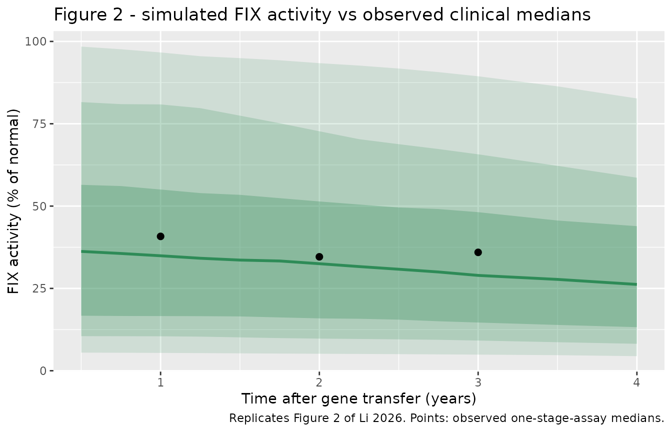
Replicate Figure 2 (first 4 years)
# Replicates Figure 2 of Li 2026: simulated median FIX activity with 50/80/95%
# intervals over the first 4 years, against the observed clinical medians.
obs_clin <- tibble(
  time = c(1, 2, 3),
  median_obs = c(40.8, 34.6, 35.95) # one-stage assay medians, Phase 2b + Phase 3
)
pop |>
  dplyr::filter(time <= 4) |>
  ggplot(aes(time, median)) +
  geom_ribbon(aes(ymin = q025, ymax = q975), alpha = 0.15, fill = "seagreen") +
  geom_ribbon(aes(ymin = q10, ymax = q90), alpha = 0.20, fill = "seagreen") +
  geom_ribbon(aes(ymin = q25, ymax = q75), alpha = 0.30, fill = "seagreen") +
  geom_line(colour = "seagreen", linewidth = 1) +
  geom_point(data = obs_clin, aes(time, median_obs), colour = "black", size = 2) +
  labs(
    x = "Time after gene transfer (years)", y = "FIX activity (% of normal)",
    title = "Figure 2 - simulated FIX activity vs observed clinical medians",
    caption = "Replicates Figure 2 of Li 2026. Points: observed one-stage-assay medians."
  )
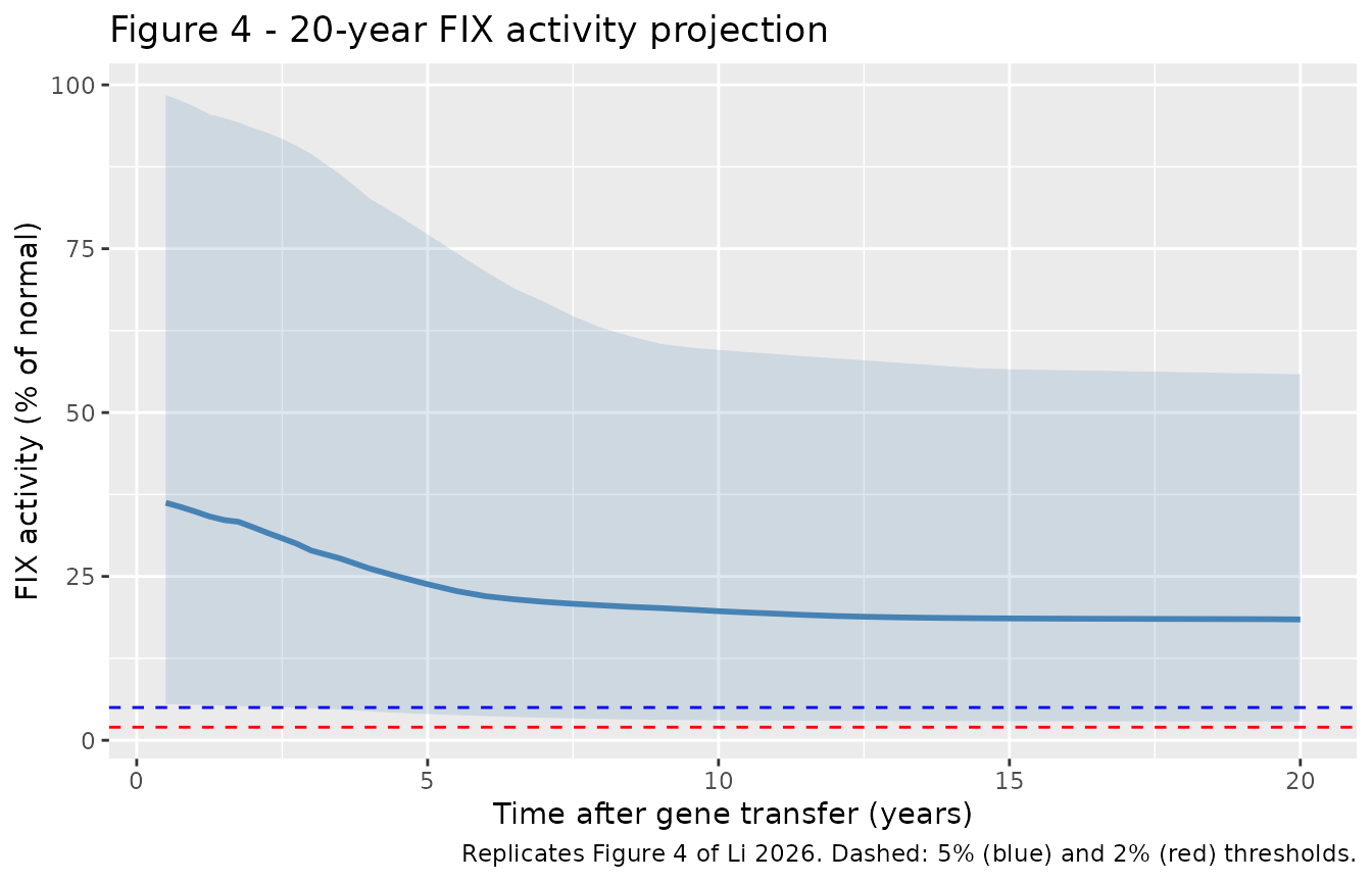
Replicate Figure 4 (20-year projection)
# Replicates Figure 4 of Li 2026: 20-year median FIX activity with 95% interval
# and the 2% / 5% durability thresholds.
ggplot(pop, aes(time, median)) +
  geom_ribbon(aes(ymin = q025, ymax = q975), alpha = 0.18, fill = "steelblue") +
  geom_line(colour = "steelblue", linewidth = 1) +
  geom_hline(yintercept = 5, linetype = "dashed", colour = "blue") +
  geom_hline(yintercept = 2, linetype = "dashed", colour = "red") +
  labs(
    x = "Time after gene transfer (years)", y = "FIX activity (% of normal)",
    title = "Figure 4 - 20-year FIX activity projection",
    caption = "Replicates Figure 4 of Li 2026. Dashed: 5% (blue) and 2% (red) thresholds."
  )
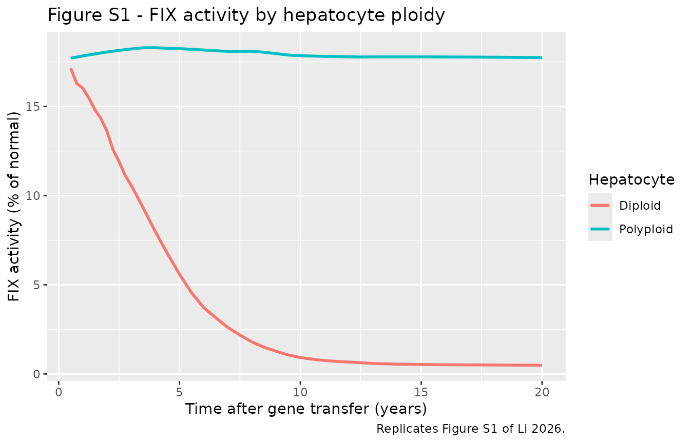
Replicate Figure S1 (diploid vs polyploid contributions)
# Replicates Figure S1 of Li 2026: FIX activity split by the hepatocyte
# population that produces it. The diploid share decays over the first ~6 years
# (fast turnover); the long-lived polyploid share sustains long-term activity.
ploidy <- sim |>
  dplyr::group_by(time) |>
  dplyr::summarise(
    Diploid = median(FIXactivity_di),
    Polyploid = median(FIXactivity_poly),
    .groups = "drop"
  ) |>
  tidyr::pivot_longer(c(Diploid, Polyploid),
    names_to = "Hepatocyte", values_to = "fix"
  )
ggplot(ploidy, aes(time, fix, colour = Hepatocyte)) +
  geom_line(linewidth = 1) +
  labs(
    x = "Time after gene transfer (years)", y = "FIX activity (% of normal)",
    title = "Figure S1 - FIX activity by hepatocyte ploidy",
    caption = "Replicates Figure S1 of Li 2026."
  )
Validation
# Published values from the Results text: medians (95% CI) at Years 1, 2, 3 and
# 20, and the Year 5 mean (95% CI).
published <- tibble(
  time = c(1, 2, 3, 5, 20),
  published_median = c(35.3, 31.8, 28.2, NA, 22.6),
  published_mean = c(NA, NA, NA, 23.5, NA),
  published_ci = c(
    "7.82-99.1", "7.01-91.7", "6.12-83.5", "4.92-72.2", "4.58-71"
  )
)
cmp <- pop |>
  dplyr::filter(time %in% c(1, 2, 3, 5, 20)) |>
  dplyr::select(time, median, mean, q025, q975) |>
  dplyr::mutate(dplyr::across(c(median, mean, q025, q975), ~ round(.x, 1))) |>
  dplyr::mutate(sim_ci = paste0(q025, "-", q975)) |>
  dplyr::left_join(published, by = "time") |>
  dplyr::select(
    time, median, published_median, mean, published_mean, sim_ci, published_ci
  )
cmp |>
  dplyr::rename(
    "Year" = time,
    "Simulated median" = median,
    "Published median" = published_median,
    "Simulated mean" = mean,
    "Published mean" = published_mean,
    "Simulated 95% interval" = sim_ci,
    "Published 95% CI" = published_ci
  ) |>
  knitr::kable(
    caption = "Simulated vs published FIX activity (% of normal), default scenario. The early-year medians and the intervals match; the later-year medians sit below the published figures for the reason given under Assumptions and deviations."
)| Year | Simulated median | Published median | Simulated mean | Published mean | Simulated 95% interval | Published 95% CI |
|---|---|---|---|---|---|---|
| 1 | 34.9 | 35.3 | 39.3 | NA | 5.4-96.7 | 7.82-99.1 |
| 2 | 32.5 | 31.8 | 36.9 | NA | 5.2-93.4 | 7.01-91.7 |
| 3 | 28.9 | 28.2 | 33.9 | NA | 4.9-89.4 | 6.12-83.5 |
| 5 | 23.8 | NA | 28.2 | 23.5 | 4-77.2 | 4.92-72.2 |
| 20 | 18.4 | 22.6 | 20.4 | NA | 2.9-55.8 | 4.58-71 |
The simulation reproduces the published median FIX activity in the first three years (Year 1 ~35%, Year 2 ~32%, Year 3 ~29%, against the published 35.3 / 31.8 / 28.2%) and the width of the published 95% intervals, and preserves the central biological finding: FIX activity plateaus well above the 2% durability threshold, sustained almost entirely by the long-lived polyploid hepatocytes.
The paper’s even-split scenario (Figure 5B) and the transduction sensitivity (Figure 5A)
The paper’s sensitivity analysis of episome passing efficiency
(Figure 5B) includes the scenario this model encodes – every episome
kept and split evenly at division (passing efficiency 1). The paper
reports its median as 38.4% at Year 1 and 19.1% at Year 20. The
transduction-efficiency analysis (Figure 5A) lowers the
Init_Episome range 10-fold, from 10-1000 to 1-100, and
reports medians of 38.4 / 26.5 / 24.7% (default range) against 34.1 /
22.1 / 19.7% (reduced range) at Years 1 / 5 / 20. Both sensitivity
analyses report a Year 1 median of 38.4% for their reference scenario,
above the 35.3% of Figure 2, so they were evidently run under a
configuration that differs from the Figure 2 / 4 runs; the comparison
below therefore uses the reduced-to-default ratio for
Figure 5A rather than the absolute values.
# Replicates the Figure 5A scenario: same cohort, Init_Episome range 1-100.
cohort_lo <- cohort |>
  dplyr::mutate(EPISOME_MEAN = EPISOME_MEAN / 10)
events_lo <- rxode2::et(times) |>
  rxode2::et(id = seq_len(n_sub)) |>
  as.data.frame() |>
  dplyr::left_join(cohort_lo, by = "id") |>
  dplyr::arrange(id, time)
sim_lo <- rxode2::rxSolve(mod, events = events_lo, returnType = "data.frame")

fig5 <- dplyr::bind_rows(
  sim |> dplyr::mutate(scenario = "10-1000"),
  sim_lo |> dplyr::mutate(scenario = "1-100")
) |>
  dplyr::group_by(scenario, time) |>
  dplyr::summarise(
    median = median(FIXactivity),
    q025 = quantile(FIXactivity, 0.025), q975 = quantile(FIXactivity, 0.975),
    .groups = "drop"
  )
ggplot(fig5, aes(time, median, colour = scenario, fill = scenario)) +
  geom_ribbon(aes(ymin = q025, ymax = q975), alpha = 0.15, colour = NA) +
  geom_line(linewidth = 1) +
  geom_hline(yintercept = 5, linetype = "dashed", colour = "blue") +
  geom_hline(yintercept = 2, linetype = "dashed", colour = "red") +
  labs(
    x = "Time after gene transfer (years)", y = "FIX activity (% of normal)",
    colour = "Initial episomes\nper transduced cell",
    fill = "Initial episomes\nper transduced cell",
    caption = "Replicates Figure 5A of Li 2026."
  )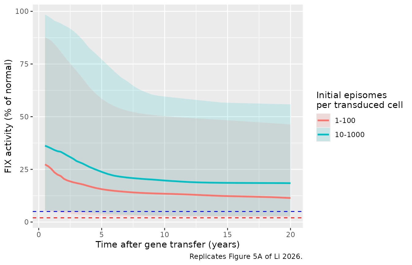
fig5_tab <- fig5 |>
  dplyr::filter(time %in% c(1, 5, 20)) |>
  dplyr::select(scenario, time, median) |>
  tidyr::pivot_wider(names_from = scenario, values_from = median) |>
  dplyr::mutate(
    sim_ratio = `1-100` / `10-1000`,
    published_even_split = c(38.4, NA, 19.1),
    published_ratio = c(34.1 / 38.4, 22.1 / 26.5, 19.7 / 24.7)
  ) |>
  dplyr::mutate(dplyr::across(-time, ~ round(.x, 3)))
fig5_tab |>
  dplyr::rename(
    "Year" = time,
    "Simulated median, 10-1000" = `10-1000`,
    "Published median, passing efficiency 1 (Fig 5B)" = published_even_split,
    "Simulated median, 1-100" = `1-100`,
    "Simulated ratio 1-100 / 10-1000" = sim_ratio,
    "Published ratio (Fig 5A)" = published_ratio
  ) |>
  knitr::kable(
    caption = "Even-split scenario and the 10-fold transduction reduction: simulated vs published."
)| Year | Simulated median, 1-100 | Simulated median, 10-1000 | Simulated ratio 1-100 / 10-1000 | Published median, passing efficiency 1 (Fig 5B) | Published ratio (Fig 5A) |
|---|---|---|---|---|---|
| 1 | 25.238 | 34.913 | 0.723 | 38.4 | 0.888 |
| 5 | 15.595 | 23.810 | 0.655 | NA | 0.834 |
| 20 | 11.391 | 18.433 | 0.618 | 19.1 | 0.798 |
The Year 20 median of this model (18.4%) sits close to the paper’s
own even-split scenario (19.1%), which supports attributing the gap to
the Figure 4 median (22.6%) to the lossy division step of the authors’
code rather than to the encoding. The 10-fold reduction in initial
episomes lowers the simulated median in the same direction as the
published Figure 5A, but by a larger proportion (simulated ratio
~0.62-0.72 vs published ~0.80-0.89): because FIX production saturates at
EPISOME_CAP episomes per cell, the reduction has more
effect in this even-split encoding, where more cells sit above the cap
in the default range than in the authors’ episome-losing code. The
direction and the sign of the sensitivity match; the magnitude reflects
the same structural difference quantified under Assumptions and
deviations.
y <- function(tt) pop[abs(pop$time - tt) < 1e-6, ]
y20 <- sim[sim$time == 20, ]
y05 <- sim[abs(sim$time - 0.5) < 1e-6, ]

stopifnot(
  # Output decomposition: total FIX activity is exactly the diploid + polyploid
  # shares (pins the reported split).
  max(abs(sim$FIXactivity - (sim$FIXactivity_di + sim$FIXactivity_poly))) < 1e-6,
  # Liver homeostasis: the total hepatocyte count stays near its initial value
  # over 20 years (no run-away growth or collapse).
  all(sim$TD + sim$TP > 0.6), all(sim$TD + sim$TP < 1.05),
  # Early-year medians track the published Figure 2 values (within a few %).
  abs(y(1)$median - 35.3) < 4,
  abs(y(2)$median - 31.8) < 4,
  abs(y(3)$median - 28.2) < 4,
  # Durability: the 20-year median stays well above the 2% prophylaxis threshold.
  y(20)$median > 5,
  # Polyploid hepatocytes sustain long-term FIX: by year 20 the polyploid share
  # exceeds the diploid share in every subject, and the diploid share has
  # collapsed relative to its early-year level.
  all(y20$FIXactivity_poly > y20$FIXactivity_di),
  median(y20$FIXactivity_di) < 0.2 * median(y05$FIXactivity_di)
)
Assumptions and deviations
Deterministic generation-ladder encoding of an agent-based model. The published model is a stochastic ABM; this file encodes its expected behaviour as a system of ordinary differential equations indexed by division count. The encoding is exact in expectation for the paper’s even-episome-split assumption and continuous rates, but it does not represent within-liver demographic stochasticity (the 1000-agent sampling noise of a single virtual liver). At the population scale used for the figures this is immaterial, because the reported intervals are dominated by the between-liver covariate variability (Table S2), which is reproduced faithfully.
Even episome split (paper text) vs the authors’ code. The maintainers encoded the paper’s stated assumption that all episomes are maintained during mitosis and split evenly between daughters (passing efficiency 1, Figure 5B). The authors’ deposited code (
AgentBased_v7.jl,CellDivide) instead gives the motherfloor(e/2)episomes and the daughterceil(floor(e/2)/2), losing roughly a quarter of episomes per division. The published figures were produced by that code.Continuous rates (paper text) vs the code’s discrete steps. Table S1 rates are encoded as continuous per-year rates, as the paper states the 0.05-year step converts the agent transition probabilities into rates. The code instead advances in discrete 0.05-year steps (death, then division). Because diploid proliferation and death nearly cancel (0.709 vs 0.726 /yr), the second-order term of the discrete scheme is not negligible for diploid cells: it roughly doubles their net turnover, so diploid hepatocytes disappear faster in the code than in the continuous model. That shrinks the total-hepatocyte denominator and raises the normalized FIX activity at later years, producing the characteristic late up-tick of Figure 4.
Size and direction of the gap. The maintainers reproduced both schemes. The two schemes agree closely for the first three years and diverge later: at 20 years the shipped even-split continuous model gives a population median of about 18%, the even-split discrete scheme about 23%, and the code’s discrete lossy-split scheme (which reproduces the published Figure 4 plateau of ~22-23%) about 21%. The discrete stepping and the lossy split push the long-term median in opposite directions, and the discrete-stepping effect dominates. The shipped model therefore tracks the published figures through Year 3 and sits a few percentage points below them from Year 5 onward; the central conclusion – a durable plateau far above the 2% threshold, sustained by polyploid hepatocytes – is unchanged.
Integer expression cap. Table S2 gives
max_episome_expressas an integer from 1 to 5, and the maintainers encoded it as such. The authors’ scan script (TwentyYear2.jl) draws it from a continuous Latin hypercube between 1 and 5 without rounding, so in the published runs the cap is a real number. The closed form for the expected expressing episomes used in the model is exact only for an integer cap; supplyEPISOME_CAPas an integer.Quasi-steady-state FIX. Per-cell FIX is taken at its within-step steady state,
min(cap, e) * kprod / kdeg, which is exactly what the code computes (the FIX half-life of ~7 h is far shorter than the dynamics). Consequently the model does not reproduce the first ~6 months of FIX accumulation after dosing; the authors likewise restricted their analysis to times later than 6 months.Population. The virtual livers represent male adults (Li 2026 Methods); the diploid-fraction-versus-age relation and the FIX-activity normalisation constants (normal plasma FIX, plasma volume, liver weight, hepatocellularity, 6x Padua potency) are taken verbatim from the Methods.
Model-specific covariate names.
TRANSDUCED_FRAC,EPISOME_MEANandEPISOME_CAPdescribe the AAV gene-therapy exposure of a virtual liver and are not epidemiological covariates in the shared register; they are documented in the model file’scovariateData.AGEis the standard register covariate.Dose. All virtual patients received the single approved dose level (
2e13genome copies/kg); dose is not an explicit model input, as the paper does not quantitatively link administered dose to the number of transduced hepatocytes.No correction notice for Li 2026 was found as of 2026-10-17.