Tigecycline (Song 2024)
Source:vignettes/articles/Song_2024_tigecycline.Rmd
Song_2024_tigecycline.RmdModel and source
- Citation: Song S, Liu J, Su W, Yu H, Feng B, Wu Y, Guo F, Yu Z. Population pharmacokinetics of tigecycline for critically ill patients undergoing continuous renal replacement therapy. Drug Des Devel Ther. 2024;18:4459-4469. doi:10.2147/DDDT.S473080
- Description: Two-compartment IV population PK model for tigecycline in critically ill adult patients undergoing continuous renal replacement therapy, with no covariates retained in the final model (Song 2024)
- Article: https://doi.org/10.2147/DDDT.S473080
Song 2024 is the CRRT-specific companion to
Su_2024_tigecycline, which the same group built on a larger
non-CRRT critically ill cohort at the same hospital. The two models
share a dosing and sampling protocol and a table layout, but not a
covariate model: Su 2024 retained five covariates, while Song 2024
retained none.
Population
Twenty-one critically ill adults contributing 167 plasma tigecycline concentrations, all receiving continuous renal replacement therapy continuously throughout tigecycline treatment (Song 2024 Table 1, which lists every patient individually). Age ranged 22-87 years (median 71), weight 42-100 kg (median 70), BMI 16.4-37.5 kg/m^2; 6 of 21 (28.6%) were female. Renal and hepatic chemistry spanned a wide range typical of an ICU cohort: serum creatinine 47-469 umol/L, BUN 3.64-37.3 mmol/L, albumin 23.0-35.7 g/L, total bilirubin 11.4-113.9 umol/L. Twenty patients received CVVH and one CVVHDF, at intensities of 21.0-51.2 mL/kg/h, anticoagulated with heparin (12), regional sodium citrate (5) or nothing (4). Residual native renal function varied from anuria to 6950 mL/24 h of urine.
The dosing and sampling schedule is not restated in this paper - the Methods point to the companion study (Su et al, Front Pharmacol 2024;15:1342947), where tigecycline was given as a 30-minute intravenous infusion every 12 h with samples immediately before the seventh dose and at 0.5, 1, 2, 3, 4, 6 and 12 h post-dose.
The same information is available programmatically via
readModelDb("Song_2024_tigecycline")()$population.
Source trace
Every ini() entry in
inst/modeldb/specificDrugs/Song_2024_tigecycline.R carries
an in-file comment naming its origin. They are collected here for
review.
| Equation / parameter | Value | Source location |
|---|---|---|
lcl |
log(4.22) |
Table 2, CL (L/h), CRRT Final Model column (RSE 10.4%;
bootstrap median 4.27, 95% CI 3.47-5.07) |
lvc |
log(30.9) |
Table 2, V1 (L) (RSE 15.9%; bootstrap median 31.6) |
lq |
log(34.8) |
Table 2, Q (L/h) (RSE 8.94%; bootstrap median
35.0) |
lvp |
log(98.7) |
Table 2, V2 (L) (RSE 11.8%; bootstrap median 98.5) |
etalcl |
0.224 |
Table 2, omega CL (%) 22.4, read as the variance (see
Assumptions) |
etalvc |
0.552 |
Table 2, omega V1 (%) 55.2, read as the variance (see
Assumptions) |
propSd |
0.1257 |
Table 2, Residual variability sigma (%) 1.58, read as
sigma^2 = 0.0158
|
| Two-compartment first-order elimination | n/a | Results, “The tigecycline concentration data could be well illustrated by a two-compartment model with first-order elimination (2425.331 and 2188.14 for the Akaike information criterion in one and two compartments, respectively)” |
| Exponential IIV, proportional residual error | n/a | Results, “An exponential model and a proportional model were used to describe the interindividual variability and residual variability, respectively” |
| No covariates | n/a | Abstract, “no covariates were found to adequately explain the [variability] in the pharmacokinetic parameters of tigecycline”; Results, AST on V2 reached significance (delta OFV 13.719) but was removed |
| 30-minute IV infusion, q12h | n/a | Methods, “The detailed study protocol was published in our previous study”; Su et al Front Pharmacol 2024;15:1342947 Methods |
| PK/PD targets AUC/MIC >= 17.9 (cSSSI), >= 12.8 (CAP), >= 6.96 (cIAI) | n/a | Methods, “Monte Carlo Simulation and Dose Regimen Evaluation” |
| Published PTA values used below | n/a | Results, “Simulation and Dosing Regimen Optimization”; Figure 3 |
Virtual cohort
The original concentrations are not public. Three cohorts of 200 subjects each are drawn, one per simulated dose regimen (50, 100 and 150 mg every 12 h - the three regimens the paper evaluated). The model retains no covariates, so a cohort is nothing but a draw from the two etas; no covariate distribution has to be reconstructed.
Steady state is imposed exactly with rxode2’s ss = 1
flag rather than approached by stacking doses. That matters here: the
peripheral volume is large (98.7 L) and IIV on V1 is wide, so a subject
in the tail of the eta distribution has a terminal half-life of days and
would still be materially short of steady state after a week of q12h
dosing. Accumulation shortfall is a physical, per-subject difference
that would corrupt the AUC identity below and vary with whichever cohort
the machine happens to draw. The paper’s own Monte Carlo simulation is a
steady-state exercise, so ss = 1 is also the matching
condition.
# set.seed() seeds R's RNG. It does NOT seed rxode2's simulation RNG, and
# rxode2's streams are partitioned PER SOLVER THREAD, so the cohort below is
# reproducible on this machine and different on a machine with a different
# thread count. Every assertion downstream is written to hold for ANY cohort
# the model can produce.
set.seed(20241005)
rxode2::rxSetSeed(20241005)

n_per_arm <- 200L
tau <- 12

# Observation grid. Dense over the distribution phase because the AUC identity
# below is a statement about trapezoidal quadrature: a subject in the low tail
# of the V1 eta has an alpha half-life of a few minutes, and a 0.1 h grid would
# leave ~1% of one-sided trapezoidal bias on such a subject. At 0.025 h the
# bias is ~0.05% for such a subject, and the realised worst case over a 600
# subject draw was 0.007% - comfortably inside the 0.5% gate, which is set with
# headroom because which V1 tail gets drawn varies with the solver thread count.
tad_obs <- sort(unique(c(seq(0, 2, by = 0.025), seq(2.1, tau, by = 0.1))))

make_arm <- function(dose, id_offset) {
  # The dose is carried as `dose_mg`, not `dose`: rxode2 reserves `dose` and
  # rejects it in `keep =` with "Cannot keep missing columns".
  subj <- tibble::tibble(
    id = id_offset + seq_len(n_per_arm),
    regimen = sprintf("%d mg q12h", dose),
    dose_mg = dose
  )
  doses <- subj |>
    dplyr::mutate(time = 0, amt = dose, evid = 1L, dur = 0.5,
                  ii = tau, ss = 1L, cmt = "central")
  obs <- subj |>
    tidyr::crossing(time = tad_obs) |>
    dplyr::mutate(amt = NA_real_, evid = 0L, dur = NA_real_,
                  ii = NA_real_, ss = NA_integer_, cmt = "central")
  dplyr::bind_rows(doses, obs) |>
    dplyr::arrange(id, time, dplyr::desc(evid))
}

regimen_doses <- c(50, 100, 150)
events <- dplyr::bind_rows(
  lapply(seq_along(regimen_doses), function(i) {
    make_arm(regimen_doses[i], id_offset = (i - 1L) * n_per_arm)
  })
)

# Disjoint IDs across arms are mandatory: rxSolve treats id as the subject key
# and would silently merge duplicated ids into one subject receiving the summed
# dose.
stopifnot(!anyDuplicated(unique(events[, c("id", "time", "evid")])))
stopifnot(dplyr::n_distinct(events$id) == 3L * n_per_arm)
Simulation
mod <- readModelDb("Song_2024_tigecycline")
# steady-state searches for long-half-life subjects exceed the default step budget
sim <- rxode2::rxSolve(mod, events = events, keep = c("regimen", "dose_mg"),
                       maxsteps = 1e6) |>
  as.data.frame()
#> ℹ parameter labels from comments will be replaced by 'label()'

# The model computes cl and vc as model variables, so rxSolve returns them per
# subject, alongside `Cc` (the individual prediction) and `sim` (that prediction
# plus a proportional residual draw). rxSolve returns observation rows only and
# does NOT return an `evid` column, so nothing downstream may filter on one.
# Fail loudly rather than silently producing an empty gate if that changes.
stopifnot(all(c("Cc", "sim", "cl", "vc", "regimen", "dose_mg") %in% names(sim)))
stopifnot(nrow(sim) == 3L * n_per_arm * length(tad_obs))
stopifnot(all(sim$Cc > 0), !anyNA(sim$Cc))
Replicate published figures
Figure 2 - concentration-time profile over a steady-state dosing interval
Song 2024 Figure 2 is a visual predictive check of plasma tigecycline
on a logarithmic concentration axis, showing observed and predicted 5th,
10th, 50th, 90th and 95th percentiles. The observed concentrations
behind it are not public, so the panel below shows only the simulated
side of that figure: the 5th / 50th / 95th percentiles of simulated
observations (individual predictions plus a proportional residual draw,
the sim column) over one steady-state dosing interval.
# Replicates the simulated percentiles of Figure 2 of Song 2024. rxSolve returns
# observation rows only, so no evid filter is needed (and none is possible -
# there is no evid column in the output).
sim |>
  dplyr::group_by(regimen, time) |>
  dplyr::summarise(
    Q05 = quantile(sim, 0.05),
    Q50 = quantile(sim, 0.50),
    Q95 = quantile(sim, 0.95),
    .groups = "drop"
  ) |>
  ggplot(aes(time, Q50)) +
  geom_ribbon(aes(ymin = Q05, ymax = Q95), alpha = 0.25) +
  geom_line() +
  facet_wrap(~regimen) +
  scale_y_log10() +
  labs(x = "Time after dose (h)", y = "Tigecycline (mg/L)",
       title = "Steady-state prediction band by regimen",
       caption = "Replicates the predicted percentiles of Figure 2 of Song 2024.")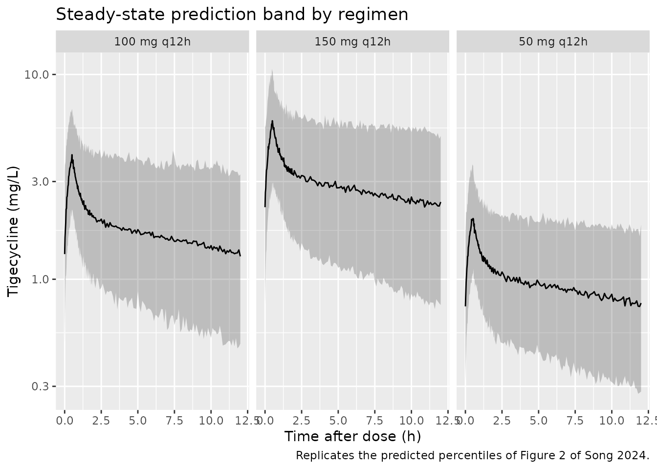
PKNCA validation
Song 2024 publishes no NCA table - no Cmax, Tmax, AUC or half-life is
reported for the cohort - so there is nothing to feed
ncaComparisonTable(). NCA is still run, for two reasons: it
produces the steady-state exposure summary a reader of this model will
want, and its AUC0-tau is the quantity the paper’s own
published outputs (the PTA and CFR analyses) are built on, so getting it
right is a precondition for the comparison in the next section.
sim_nca <- sim |>
  dplyr::filter(!is.na(Cc)) |>
  dplyr::select(id, time, Cc, regimen)

# Guarantee a time = 0 row per subject so PKNCA can anchor AUC0-tau. At exact
# steady state the trough concentration is the true value at time 0, so the row
# is already present; the bind_rows + distinct pattern is a defensive no-op
# here rather than an imputation.
sim_nca <- dplyr::bind_rows(
  sim_nca,
  sim_nca |> dplyr::distinct(id, regimen) |> dplyr::mutate(time = 0, Cc = 0)
) |>
  dplyr::distinct(id, regimen, time, .keep_all = TRUE) |>
  dplyr::arrange(id, regimen, time)

conc_obj <- PKNCA::PKNCAconc(as.data.frame(sim_nca), Cc ~ time | regimen + id)

dose_df <- events |>
  dplyr::filter(evid == 1) |>
  dplyr::select(id, time, amt, regimen) |>
  as.data.frame()
dose_obj <- PKNCA::PKNCAdose(dose_df, amt ~ time | regimen + id)

intervals <- data.frame(
  start = 0, end = tau,
  cmax = TRUE, tmax = TRUE, cmin = TRUE, auclast = TRUE, cav = TRUE
)

nca_res <- PKNCA::pk.nca(PKNCA::PKNCAdata(conc_obj, dose_obj, intervals = intervals))
nca_tbl <- as.data.frame(nca_res$result)
nca_tbl |>
  dplyr::filter(PPTESTCD %in% c("cmax", "cmin", "cav", "auclast", "tmax")) |>
  dplyr::group_by(regimen, PPTESTCD) |>
  dplyr::summarise(median = median(PPORRES),
                   p05 = quantile(PPORRES, 0.05),
                   p95 = quantile(PPORRES, 0.95),
                   .groups = "drop") |>
  tidyr::pivot_longer(c(median, p05, p95)) |>
  tidyr::pivot_wider(names_from = name, values_from = value) |>
  dplyr::rename("Regimen" = regimen, "Parameter" = PPTESTCD,
                "Median" = median, "5th pctile" = p05, "95th pctile" = p95) |>
  knitr::kable(
    digits = 2,
    caption = paste(
      "Simulated steady-state NCA over one 12 h dosing interval.",
      "Cmax / Cmin / Cav in mg/L, AUC0-12 in mg*h/L, Tmax in h.",
      "Song 2024 publishes no NCA table to compare against."
    )
)| Regimen | Parameter | Median | 5th pctile | 95th pctile |
|---|---|---|---|---|
| 100 mg q12h | auclast | 23.59 | 12.08 | 49.45 |
| 100 mg q12h | cav | 1.97 | 1.01 | 4.12 |
| 100 mg q12h | cmax | 3.91 | 2.33 | 7.00 |
| 100 mg q12h | cmin | 1.53 | 0.66 | 3.60 |
| 100 mg q12h | tmax | 0.50 | 0.50 | 0.50 |
| 150 mg q12h | auclast | 35.15 | 18.05 | 73.48 |
| 150 mg q12h | cav | 2.93 | 1.50 | 6.12 |
| 150 mg q12h | cmax | 6.23 | 3.45 | 11.04 |
| 150 mg q12h | cmin | 2.30 | 0.92 | 5.57 |
| 150 mg q12h | tmax | 0.50 | 0.50 | 0.50 |
| 50 mg q12h | auclast | 11.49 | 6.02 | 25.81 |
| 50 mg q12h | cav | 0.96 | 0.50 | 2.15 |
| 50 mg q12h | cmax | 2.02 | 1.08 | 3.51 |
| 50 mg q12h | cmin | 0.74 | 0.29 | 1.91 |
| 50 mg q12h | tmax | 0.50 | 0.50 | 0.50 |
Gate 1 - AUC0-tau at steady state equals Dose / CL
Both sides of this check use the same drawn parameters, so the only difference is trapezoidal discretisation of a convex curve. That is one-sided (every subject should come out slightly high) and a tight bound is the correct assertion here - unlike a cohort-extreme bound, it does not depend on which subjects were drawn.
cl_by_id <- sim |>
  dplyr::group_by(regimen, id, dose_mg) |>
  dplyr::summarise(cl = dplyr::first(cl), .groups = "drop")

auc_chk <- nca_tbl |>
  dplyr::filter(PPTESTCD == "auclast") |>
  dplyr::select(regimen, id, auc_nca = PPORRES) |>
  dplyr::inner_join(cl_by_id, by = c("regimen", "id")) |>
  dplyr::mutate(auc_closed = dose_mg / cl,
                pct_diff = 100 * (auc_nca - auc_closed) / auc_closed)

stopifnot(nrow(auc_chk) == 3L * n_per_arm)   # a gate with no rows cannot go red
stopifnot(max(abs(auc_chk$pct_diff)) < 0.5)
# No assertion on the SIGN of the bias: trapezoidal over-reading of a convex
# curve is one-sided in principle, but at 0.007% the residual is down in solver
# noise, and asserting the sign of a near-zero quantity is exactly the shape
# that passes locally and fails in CI.

sprintf("AUC0-12,ss vs dose/CL: max |%% diff| = %.3f%% over %d subjects",
        max(abs(auc_chk$pct_diff)), nrow(auc_chk))
#> [1] "AUC0-12,ss vs dose/CL: max |% diff| = 0.017% over 600 subjects"
Comparison against published results
The paper’s published quantitative outputs are its probability-of-target- attainment analysis (Results text and Figure 3) and its cumulative fraction of response analysis (Figure 4). The CFR figures cannot be reproduced here: they weight the PTA curve by EUCAST MIC distributions that live in Supplementary Tables S2 and S3, which are not distributed through PubMed Central. The PTA values are reproducible, and are used below.
At steady state AUC0-24 = 2 * Dose / CL exactly, and CL
is log-normal, so PTA has a closed form:
PTA(dose, target, MIC) = Phi( log( (2 * dose / CL_typ) / (target * MIC) ) / omega_CL )
That closed form is the discriminating leg (it is deterministic and immune to which cohort the machine draws); the simulated cohort is checked against it first, so that sampling noise and model-versus-paper disagreement cannot mask each other.
ui <- rxode2::rxode(mod)
#> ℹ parameter labels from comments will be replaced by 'label()'
theta <- setNames(ui$theta, names(ui$theta))
cl_typ <- exp(theta[["lcl"]])
omega_cl <- sqrt(ui$omega["etalcl", "etalcl"])

pta_closed <- function(dose, target, mic, omega = omega_cl) {
  stats::pnorm(log((2 * dose / cl_typ) / (target * mic)) / omega) * 100
}

targets <- c(cSSSI = 17.9, CAP = 12.8, cIAI = 6.96)

sprintf("CL_typ = %.2f L/h; omega_CL (log-scale SD) = %.4f", cl_typ, omega_cl)
#> [1] "CL_typ = 4.22 L/h; omega_CL (log-scale SD) = 0.4733"
Gate 2 - the simulated cohort reproduces the closed form
mic_grid <- 2^seq(-3, 6)   # 0.125 to 64 mg/L, the axis of Figure 3

pta_sim <- tidyr::crossing(
  cl_by_id |> dplyr::select(regimen, id, dose_mg, cl),
  MIC = mic_grid,
  infection = names(targets)
) |>
  dplyr::mutate(target = unname(targets[infection]),
                auc24 = 2 * dose_mg / cl,
                hit = auc24 / MIC >= target) |>
  dplyr::group_by(regimen, dose_mg, infection, target, MIC) |>
  dplyr::summarise(pta_sim = 100 * mean(hit), .groups = "drop") |>
  dplyr::mutate(pta_cf = pta_closed(dose_mg, target, MIC))

stopifnot(nrow(pta_sim) == 3L * length(mic_grid) * length(targets))

# 200 subjects per arm: a binomial proportion near 50% carries a standard error
# of 3.5 points, so ~11 points is a 3-SE envelope. The bound is on the MAXIMUM
# over 90 cells, which is why it is not tighter; it still goes red on any
# mis-encoded omega (the CV reading below moves cells by 30+ points).
stopifnot(max(abs(pta_sim$pta_sim - pta_sim$pta_cf)) < 15)
stopifnot(mean(abs(pta_sim$pta_sim - pta_sim$pta_cf)) < 5)

sprintf("Cohort vs closed-form PTA: max = %.1f points, mean = %.1f points over %d cells",
        max(abs(pta_sim$pta_sim - pta_sim$pta_cf)),
        mean(abs(pta_sim$pta_sim - pta_sim$pta_cf)),
        nrow(pta_sim))
#> [1] "Cohort vs closed-form PTA: max = 4.2 points, mean = 0.5 points over 90 cells"
Figure 3 - probability of target attainment versus MIC
# Replicates Figure 3 of Song 2024: PTA vs MIC for the three PK/PD targets,
# one curve per dose regimen.
pta_sim |>
  dplyr::mutate(
    panel = factor(
      infection,
      levels = c("cSSSI", "CAP", "cIAI"),
      labels = c("A: cSSSI, AUC/MIC >= 17.9",
                 "B: CAP, AUC/MIC >= 12.8",
                 "C: cIAI, AUC/MIC >= 6.96")
    )
  ) |>
  ggplot(aes(MIC, pta_sim, colour = regimen)) +
  geom_hline(yintercept = 90, linetype = "dotted") +
  geom_line() +
  geom_point() +
  facet_wrap(~panel, ncol = 1) +
  scale_x_log10(breaks = mic_grid, labels = mic_grid) +
  labs(x = "MIC (mg/L)", y = "PTA (%)", colour = NULL,
       title = "Probability of target attainment by regimen",
       caption = "Replicates Figure 3 of Song 2024.")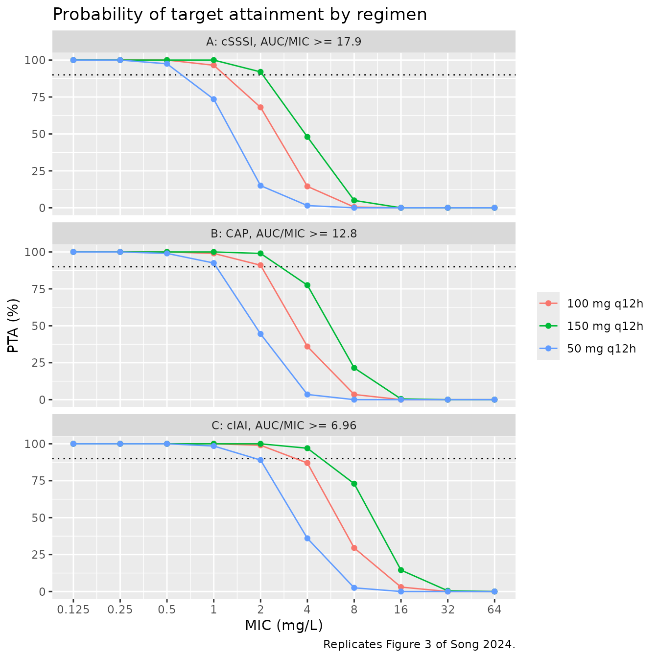
Gate 3 - closed form versus the published PTA values
The six PTA values printed in the Results section are transcribed below and compared against the closed form. This is the deterministic leg: no cohort is involved, so the numbers are identical on every machine.
published_pta <- tibble::tribble(
  ~infection, ~dose, ~MIC, ~pta_pub,
  "cSSSI",       50,    1,     58.2,
  "cSSSI",      100,    1,     98.1,
  "CAP",         50,    1,     85.0,
  "CAP",        100,    1,     99.9,
  "cIAI",        50,    2,     82.4,
  "cIAI",       100,    2,     99.7
) |>
  dplyr::mutate(target = unname(targets[infection]),
                pta_model = pta_closed(dose, target, MIC),
                diff = pta_model - pta_pub)

published_pta |>
  dplyr::transmute(
    "Infection" = infection,
    "Regimen" = sprintf("%d mg q12h", dose),
    "MIC (mg/L)" = MIC,
    "Target AUC0-24/MIC" = target,
    "Published PTA (%)" = pta_pub,
    "Model PTA (%)" = round(pta_model, 1),
    "Difference (points)" = round(diff, 1)
  ) |>
  knitr::kable(
    caption = paste(
      "Published PTA (Song 2024 Results) against the closed form implied by the",
      "packaged model. Deterministic - no simulated cohort is involved."
    )
)| Infection | Regimen | MIC (mg/L) | Target AUC0-24/MIC | Published PTA (%) | Model PTA (%) | Difference (points) |
|---|---|---|---|---|---|---|
| cSSSI | 50 mg q12h | 1 | 17.90 | 58.2 | 72.3 | 14.1 |
| cSSSI | 100 mg q12h | 1 | 17.90 | 98.1 | 98.0 | -0.1 |
| CAP | 50 mg q12h | 1 | 12.80 | 85.0 | 90.3 | 5.3 |
| CAP | 100 mg q12h | 1 | 12.80 | 99.9 | 99.7 | -0.2 |
| cIAI | 50 mg q12h | 2 | 6.96 | 82.4 | 87.0 | 4.6 |
| cIAI | 100 mg q12h | 2 | 6.96 | 99.7 | 99.5 | -0.2 |
# Deterministic quantity, so a tight bound is correct. The three 100 mg cells
# land within 0.2 points; the 50 mg cells read high (see Assumptions), with
# cSSSI the worst at ~14 points.
stopifnot(nrow(published_pta) == 6L)
stopifnot(mean(abs(published_pta$diff)) < 6)
stopifnot(max(abs(published_pta$diff[published_pta$dose == 100])) < 1)

sprintf("Published vs closed-form PTA: mean |difference| = %.2f points",
        mean(abs(published_pta$diff)))
#> [1] "Published vs closed-form PTA: mean |difference| = 4.08 points"
Gate 4 - the omega scale, adjudicated against the paper’s own simulation
Table 2 prints the between-subject terms as
omega CL (%) 22.4 and omega V1 (%) 55.2. Two
readings are possible: coefficients of variation, or NONMEM OMEGA
variances written as percentages. The choice changes the
log-scale SD of CL by a factor of two, so it is worth settling from
evidence.
Inverting the six published PTA values through the standard normal
recovers the median steady-state AUC0-24 that the authors’
own Monte Carlo simulation must have produced. Under the correct reading
that number has to agree with 2 * Dose / CL computed from
the CL in the same table. This uses no free parameters and no
digitisation.
omega_variance <- sqrt(0.224)                    # Table 2 value read as omega^2
omega_cv       <- sqrt(log(0.224^2 + 1))         # Table 2 value read as a CV

score_reading <- function(omega, label) {
  d <- published_pta |>
    dplyr::mutate(
      z = stats::qnorm(pta_pub / 100),
      # Median AUC0-24 for a 50 mg q12h regimen implied by this PTA cell.
      log_auc50 = z * omega + log(target * MIC) - log(dose / 50)
    )
  auc_implied <- exp(mean(d$log_auc50))
  auc_nominal <- 2 * 50 / cl_typ
  fitted <- pta_closed(d$dose, d$target, d$MIC, omega = omega)
  tibble::tibble(
    Reading = label,
    "omega_CL (log-scale SD)" = round(omega, 4),
    "Implied median AUC0-24 at 50 mg q12h" = round(auc_implied, 2),
    "2 x Dose / CL from Table 2" = round(auc_nominal, 2),
    "Miss (%)" = round(100 * (auc_implied / auc_nominal - 1), 1),
    "Mean |PTA error| (points)" = round(mean(abs(fitted - d$pta_pub)), 2)
  )
}

omega_score <- dplyr::bind_rows(
  score_reading(omega_variance, "Table 2 value is omega^2 (encoded)"),
  score_reading(omega_cv,       "Table 2 value is a CV (rejected)")
)

knitr::kable(
  omega_score,
  caption = paste(
    "Adjudicating the omega scale against the paper's own printed PTA values.",
    "The variance reading recovers the paper's own CL; the CV reading does not."
  )
)| Reading | omega_CL (log-scale SD) | Implied median AUC0-24 at 50 mg q12h | 2 x Dose / CL from Table 2 | Miss (%) | Mean |PTA error| (points) |
|---|---|---|---|---|---|
| Table 2 value is omega^2 (encoded) | 0.4733 | 23.06 | 23.7 | -2.7 | 4.08 |
| Table 2 value is a CV (rejected) | 0.2213 | 15.10 | 23.7 | -36.3 | 10.90 |
var_row <- omega_score[1, ]
cv_row  <- omega_score[2, ]

# Deterministic. The variance reading must recover the paper's own AUC0-24 to
# within 10%, must beat the CV reading on PTA error, and the CV reading must
# miss the AUC0-24 anchor by more than 25% - i.e. the two readings must be
# separated, not merely ranked.
stopifnot(abs(var_row[["Miss (%)"]]) < 10)
stopifnot(abs(cv_row[["Miss (%)"]]) > 25)
stopifnot(var_row[["Mean |PTA error| (points)"]] <
            cv_row[["Mean |PTA error| (points)"]])
Assumptions and deviations
-
The between-subject terms in Table 2 are variances, not
coefficients of variation. Table 2 heads its variability block
omega CL (%),omega V1 (%)andResidual variability sigma (%), printing 22.4, 55.2 and 1.58. Read literally as coefficients of variation the residual row is a 1.58% proportional error, which is below the precision of the LC-MS/MS assay itself and is contradicted by the scatter in the paper’s own Figure 1 DV-versus-IPRED panel. The whole block is therefore read on the NONMEM variance scale (omega^2 = 0.224and0.552,sigma^2 = 0.0158), giving log-scale SDs of 0.473 and 0.743 andpropSd = 0.126. Gate 4 above settles theomegarows quantitatively with no free parameters: inverting the six published PTA values recovers a median steady-stateAUC0-24of 23.06 mgh/L under the variance reading against2 x 50 mg / 4.22 L/h = 23.7, a 2.7% miss, versus 15.1 mgh/L under the CV reading, a 36% miss; and the variance reading reproduces the printed PTAs to a mean absolute error of 4.1 percentage points versus 10.9. The direction is also the physically expected one: this model retains no covariates at all, so its unexplained IIV on CL (50% CV under the variance reading) should exceed - not fall below - the 27% reported by the same group’s five-covariate non-CRRT model. -
This differs from how the same table format is encoded in
Su_2024_tigecycline. That model, extracted earlier from the companion paper, reads the identicalomega (%)rows as coefficients of variation while readingsigma (%)as a variance. Its own vignette records the choice as unresolved (“the coefficient-of-variation reading is slightly too narrow at late times and the variance reading is clearly too wide”, from a digitised VPC) and warns that any use depending on the magnitude of between-subject variability should treat it as uncertain. Song 2024 supplies stronger evidence than Su 2024 had available - printed PTA values rather than digitised curves, and an independent anchor in the form of the paper’s own CL - so this extraction follows that evidence. The two models are consequently on different omega conventions, and reconciling them is worth a follow-up onSu_2024_tigecycline. - The 50 mg PTA cells read 4.6 to 14.1 points high; the 100 mg cells land within 0.2 points. Under the encoded model the published PTAs at 50 mg q12h reproduce as 72.3 / 90.3 / 87.0 against the printed 58.2 / 85.0 / 82.4, while at 100 mg q12h they reproduce as 98.0 / 99.7 / 99.5 against 98.1 / 99.9 / 99.7. Fitting both the median AUC and the spread freely to the six printed values gives a log-scale SD near 0.36 rather than 0.47, so the paper’s own simulated PTA curves are slightly steeper than the Table 2 omega implies. The paper does not say how many doses its Monte Carlo simulation ran for, nor how AUC was computed from the simulated profiles, so the residual is not attributable. It is recorded here rather than tuned away; no parameter has been adjusted to close it.
- The Abstract’s clearance is a transcription slip. The Abstract states “The typical values of CL, Q, V1 and V2 were 4.42 L/h, 34.8 L/h, 30.9 L and 98.7 L”, agreeing with Table 2 on three of four. Table 2 (4.22, RSE 10.4%), the bootstrap median (4.27, 95% CI 3.47-5.07) and the Discussion (“4.22 L/h, 34.8 L/h, 30.9 L and 98.7 L”) all give 4.22 L/h. The model uses 4.22.
-
Figure 3 panel C’s axis label misprints the cIAI
target. The panel C y-axis reads
AUC/MIC >= 6.69while the Methods, the figure caption and the Discussion all give 6.96. 6.96 is used. -
Table 2’s footnote misprints the companion paper’s article
number. The note cites “Su et al, Front Pharm. 2024, 15:
1342954” for the non-CRRT column; the paper’s own reference list
(reference 14) gives Front Pharmacol 2024;15:1342947, which is
the article that exists and the one
Su_2024_tigecyclineis built from. -
The non-CRRT column of Table 2 is not extracted
here. Those estimates (CL 3.09 L/h, V1 32.1 L, Q 39.7 L/h, V2
113 L) are reprinted from the companion Su et al study and are already
packaged, with their covariate model, as
Su_2024_tigecycline. Only the CRRT final model is new in this paper. -
AST is documented as screened but not encoded. AST
on V2 was the one covariate to clear forward inclusion (delta OFV
13.719) before the authors removed it. Neither the effect form nor its
coefficient is printed anywhere in the paper - only the delta OFV - so
the relationship could not be reconstructed even if a user wanted it. It
is recorded in the model’s
covariatesDataExcludedlist along with the rest of the screened covariates. -
The infusion duration comes from the companion
paper. Song 2024 does not restate the administration or
sampling schedule, pointing instead to its previous study. The 30-minute
q12h intravenous infusion used in the simulations above is from Su et al
Front Pharmacol 2024;15:1342947 Methods, the study Song 2024
cites as its protocol source. Because the model is linear, the
steady-state
AUC0-taugates are insensitive to this choice; the Cmax and Tmax rows of the NCA summary are not. -
Steady state is imposed rather than approached. The
simulations use
ss = 1so that each subject is solved at its own exact periodic steady state. Stacking a finite number of q12h doses instead would leave subjects in the tail of the V1 eta distribution materially short of steady state, making the AUC identity a statement about accumulation rather than about quadrature, and making it depend on which cohort the machine drew. - Supplementary Tables S1-S3 are not available. S1 (covariate screening progression), S2 and S3 (PTA and CFR tabulations with the EUCAST MIC distributions) are cited in the text but are not distributed through PubMed Central (the only files deposited with PMC11464410 are the article figures). No parameter in the model file depends on them. The consequence is that the CFR analysis of Figure 4 cannot be reproduced, since the pathogen-specific MIC distributions it weights by are in S3.
- No covariate distribution had to be assumed. The final model retains no covariates, so the virtual cohorts are pure draws from the two etas and no demographic distribution needed reconstructing from Table 1.