Cefathiamidine in infants with augmented renal clearance (Du 2021)

Model and source

mod <- readModelDb("Du_2021_cefathiamidine")
mod_ui <- rxode2::rxode2(mod)
#> ℹ parameter labels from comments will be replaced by 'label()'
mod_meta <- mod_ui$meta

• Citation: Du B, Zhou Y, Tang BH, Wu YE, Yang XM, Shi HY, Yao BF, Hao GX, You DP, van den Anker J, Zheng Y, Zhao W. Population Pharmacokinetic Study of Cefathiamidine in Infants With Augmented Renal Clearance. Front Pharmacol. 2021;12:630047. doi:10.3389/fphar.2021.630047.
• Description: One-compartment IV population PK model for cefathiamidine in infants 0.35-1.86 years with augmented renal clearance (Du 2021), with fixed allometric body-weight scaling on CL and V (reference 10.25 kg) and a power-form age effect on CL (reference 1.25 years).
• Article (DOI): https://doi.org/10.3389/fphar.2021.630047

Du 2021 developed a one-compartment population PK model for intravenous cefathiamidine, a first-generation cephalosporin used widely in Chinese paediatrics, in 20 infants with augmented renal clearance (ARC). Clearance scales allometrically with current body weight (fixed exponent 0.75) and additionally rises with age through a power function; volume scales linearly with weight. The paper then used Monte Carlo simulation to show that the prescribed 100 mg/kg/day q12h regimen reaches the 70% fT > MIC target only for MIC <= 0.25 mg/L, and recommended 50 mg/kg/day q8h and 75 mg/kg/day q6h for MICs of 0.5 and 2 mg/L.

This vignette validates the packaged model against the paper’s Table 2 parameter estimates, its reported weight-normalised clearance and volume, the age-group clearance contrast in the Discussion, and the probability of target attainment (PTA) values quoted in the Results text for Figure 2.

A companion model for older children, fitted by the same group, is Zhi_2018_cefathiamidine (two compartments, weight only; 54 children 2-12 years with haematological disease).

Population

Du 2021 enrolled 20 Chinese infants (10 male, 10 female) aged 0.35-1.86 years (mean 1.20, SD 0.43; median 1.25) and weighing 8.0-13.0 kg (mean 10.33, SD 1.57; median 10.25) at the Children’s Hospital of Hebei Province. All had ARC, defined as a Schwartz eGFR >= 130 mL/min/1.73 m^2 (median 197, range 132-413), and haematological disease (immune thrombocytopenia 6, leukaemia 3, anaemia 3, infectious mononucleosis syndrome 2, agranulocytosis 2, other 4). Every infant received cefathiamidine 100 mg/kg/day q12h as a 30-minute intravenous infusion (median 50 mg/kg per dose, range 40-100). Thirty-six scavenged plasma samples (0.15-222 ug/mL, all above the 30 ng/mL LLOQ) were analysed in NONMEM 7.4 with FOCE-I. Source: Du 2021 Methods and Table 1.

str(mod_meta$population)
#> List of 14
#>  $ species       : chr "human"
#>  $ n_subjects    : int 20
#>  $ n_studies     : int 1
#>  $ age_range     : chr "0.35-1.86 years"
#>  $ age_median    : chr "1.25 years"
#>  $ weight_range  : chr "8.0-13.0 kg"
#>  $ weight_median : chr "10.25 kg"
#>  $ sex_female_pct: num 50
#>  $ race_ethnicity: chr "Chinese (Du 2021 Table 1)"
#>  $ disease_state : chr "Infants (<= 2 years) with augmented renal clearance (Schwartz eGFR >= 130 mL/min/1.73 m^2) and hematologic dise"| __truncated__
#>  $ dose_range    : chr "100 mg/kg/day cefathiamidine IV q12h as a 30-min infusion (median 50 mg/kg/dose, range 40-100; median 500 mg/do"| __truncated__
#>  $ regions       : chr "China (Children's Hospital of Hebei Province, Shijiazhuang; single centre)"
#>  $ renal_function: chr "eGFR (Schwartz) median 197 mL/min/1.73 m^2 (range 132-413); serum creatinine median 20 umol/L (range 10-26)"
#>  $ notes         : chr "Baseline demographics per Du 2021 Table 1. 36 scavenged plasma samples (0.15-222 ug/mL, all above the 30 ng/mL "| __truncated__

Source trace

Every ini() value carries an in-file comment naming its source. They are collected here.

Parameter / equation	Value	Source location
lcl (CL at 10.25 kg, 1.25 years)	log(2.20) L/h	Table 2, theta_1 = 2.20 (RSE 8.30%)
lvc (V at 10.25 kg)	log(3.36) L	Table 2, theta_2 = 3.36 (RSE 8.2%)
e_wt_cl	fixed(0.75)	Methods and Results, Covariate Analysis: fixed allometric exponent 0.75 for CL; Table 2 CL formula
e_wt_vc	fixed(1)	Methods and Results, Covariate Analysis: fixed exponent 1 for V; Table 2 V formula
e_age_cl	0.662	Table 2, theta_3 = 0.662 (RSE 21.6%) in F_age = (AGE/1.25)^theta_3
etalcl ~ 0.063478	log(0.256^2 + 1)	Table 2, IIV CL 25.6% (shrinkage 15.1%)
etalvc ~ 0.048958	log(0.224^2 + 1)	Table 2, IIV V 22.4% (shrinkage 28.5%)
expSd <- 0.223191	sqrt(log(0.226^2 + 1))	Table 2, ERR(1) 22.6% (shrinkage 35.4%); Results: exponential residual model
cl <- exp(lcl + etalcl) * (WT/10.25)^e_wt_cl * (AGE/1.25)^e_age_cl		Table 2 CL formula and footnote (10.25 kg and 1.25 years are the cohort medians)
vc <- exp(lvc + etalvc) * (WT/10.25)^e_wt_vc		Table 2 V formula
d/dt(central) <- -kel * central		Results, Model Building: one-compartment model with first-order elimination
Cc ~ lnorm(expSd)		Results, Model Building: exponential residual variability
Individual parameters		Methods: theta_i = theta * exp(eta_i)

Typical-value checks

At the reference infant (10.25 kg, 1.25 years) the model gives the Table 2 typical values directly. Dividing by 10.25 kg gives weight-normalised values that the paper summarises as a median over the 20 infants of 0.22 L/h/kg (clearance) and 0.34 L/kg (volume).

typ <- data.frame(
  quantity = c("CL/WT (L/h/kg)", "V/WT (L/kg)"),
  model_reference_infant = c(2.20 / 10.25, 3.36 / 10.25),
  paper_cohort_median = c(0.22, 0.34)
) |>
  mutate(pct_diff = 100 * (model_reference_infant / paper_cohort_median - 1))
knitr::kable(typ, digits = 3)

quantity	model_reference_infant	paper_cohort_median	pct_diff
CL/WT (L/h/kg)	0.215	0.22	-2.439
V/WT (L/kg)	0.328	0.34	-3.587

# A mis-transcribed theta or reference weight moves these by tens of percent.
stopifnot(all(abs(typ$pct_diff) < 5))

Virtual cohort

The individual data are not public. The cohort below reproduces the Table 1 summaries: weight and age drawn from normal distributions with the published means and SDs (the Results report both as normally distributed, Kolmogorov-Smirnov p = 0.20 and 0.08), redrawn when outside the observed ranges. Random effects are drawn with base R from the model’s omega and passed to the solver as data, so every number in this vignette is fixed by set.seed() and does not depend on the rxode2 random-number stream.

The paper simulated 1,000 virtual infants for its PTA analysis. The same 1,000 are used here for the closed-form PTA calculation below; the first 200 of them are also solved with rxSolve() per regimen.

set.seed(20210315)
n_cohort <- 1000L

draw_truncated <- function(n, mean, sd, lower, upper) {
  x <- rnorm(n, mean, sd)
  out <- x < lower | x > upper
  while (any(out)) {
    x[out] <- rnorm(sum(out), mean, sd)
    out <- x < lower | x > upper
  }
  x
}

omega <- mod_ui$omega
cohort <- tibble(
  id = seq_len(n_cohort),
  WT = draw_truncated(n_cohort, 10.33, 1.57, 8.0, 13.0),
  AGE = draw_truncated(n_cohort, 1.20, 0.43, 0.35, 1.86),
  etalcl = rnorm(n_cohort, 0, sqrt(omega["etalcl", "etalcl"])),
  etalvc = rnorm(n_cohort, 0, sqrt(omega["etalvc", "etalvc"]))
) |>
  mutate(
    cl = 2.20 * (WT / 10.25)^0.75 * (AGE / 1.25)^0.662 * exp(etalcl),
    vc = 3.36 * (WT / 10.25) * exp(etalvc)
  )

summary(cohort[, c("WT", "AGE")])
#>        WT              AGE        
#>  Min.   : 8.005   Min.   :0.3556  
#>  1st Qu.: 9.443   1st Qu.:0.9215  
#>  Median :10.397   Median :1.1859  
#>  Mean   :10.404   Mean   :1.1730  
#>  3rd Qu.:11.329   3rd Qu.:1.4554  
#>  Max.   :12.996   Max.   :1.8597

Weight-normalised clearance and the age effect

The Results give the median (range) of the individual weight-normalised clearance as 0.22 (0.09-0.29) L/h/kg and volume as 0.34 (0.24-0.41) L/kg. Those are empirical Bayes estimates for 20 infants, shrunk toward the typical value (shrinkage 15.1% and 28.5%), so the simulated cohort, which carries the full between-subject variability, is expected to have similar centres and wider ranges.

The Discussion also reports mean (SD) clearance of 0.11 (0.032) L/h/kg for infants <= 1 year and 0.23 (0.034) L/h/kg for infants aged 1-2 years.

norm_tab <- cohort |>
  summarise(
    `CL/WT median` = median(cl / WT),
    `CL/WT 5th` = quantile(cl / WT, 0.05),
    `CL/WT 95th` = quantile(cl / WT, 0.95),
    `V/WT median` = median(vc / WT),
    `V/WT 5th` = quantile(vc / WT, 0.05),
    `V/WT 95th` = quantile(vc / WT, 0.95)
  )
knitr::kable(norm_tab, digits = 3)

CL/WT median	CL/WT 5th	CL/WT 95th	V/WT median	V/WT 5th	V/WT 95th
0.202	0.113	0.327	0.327	0.229	0.47

age_tab <- cohort |>
  mutate(age_group = factor(
    if_else(AGE <= 1, "<= 1 year", "1-2 years"),
    levels = c("<= 1 year", "1-2 years")
  )) |>
  group_by(age_group) |>
  summarise(n = n(), mean_cl_per_kg = mean(cl / WT), sd_cl_per_kg = sd(cl / WT)) |>
  mutate(paper_mean = c(0.11, 0.23))
stopifnot(identical(as.character(age_tab$age_group), c("<= 1 year", "1-2 years")))
knitr::kable(age_tab, digits = 3)

age_group	n	mean_cl_per_kg	sd_cl_per_kg	paper_mean
<= 1 year	329	0.157	0.044	0.11
1-2 years	671	0.234	0.063	0.23

stopifnot(
  # Centre of the cohort against the paper's median.
  abs(norm_tab$`CL/WT median` / 0.22 - 1) < 0.15,
  abs(norm_tab$`V/WT median` / 0.34 - 1) < 0.10,
  # The 1-2 year group, where most of the cohort sits, matches the paper.
  abs(age_tab$mean_cl_per_kg[2] / 0.23 - 1) < 0.10,
  # Direction of the age effect: younger infants clear less per kg.
  age_tab$mean_cl_per_kg[2] / age_tab$mean_cl_per_kg[1] > 1.2
)

ggplot(cohort, aes(AGE, cl / WT)) +
  geom_point(alpha = 0.3) +
  labs(x = "Age (years)", y = "CL / WT (L/h/kg)") +
  theme_bw()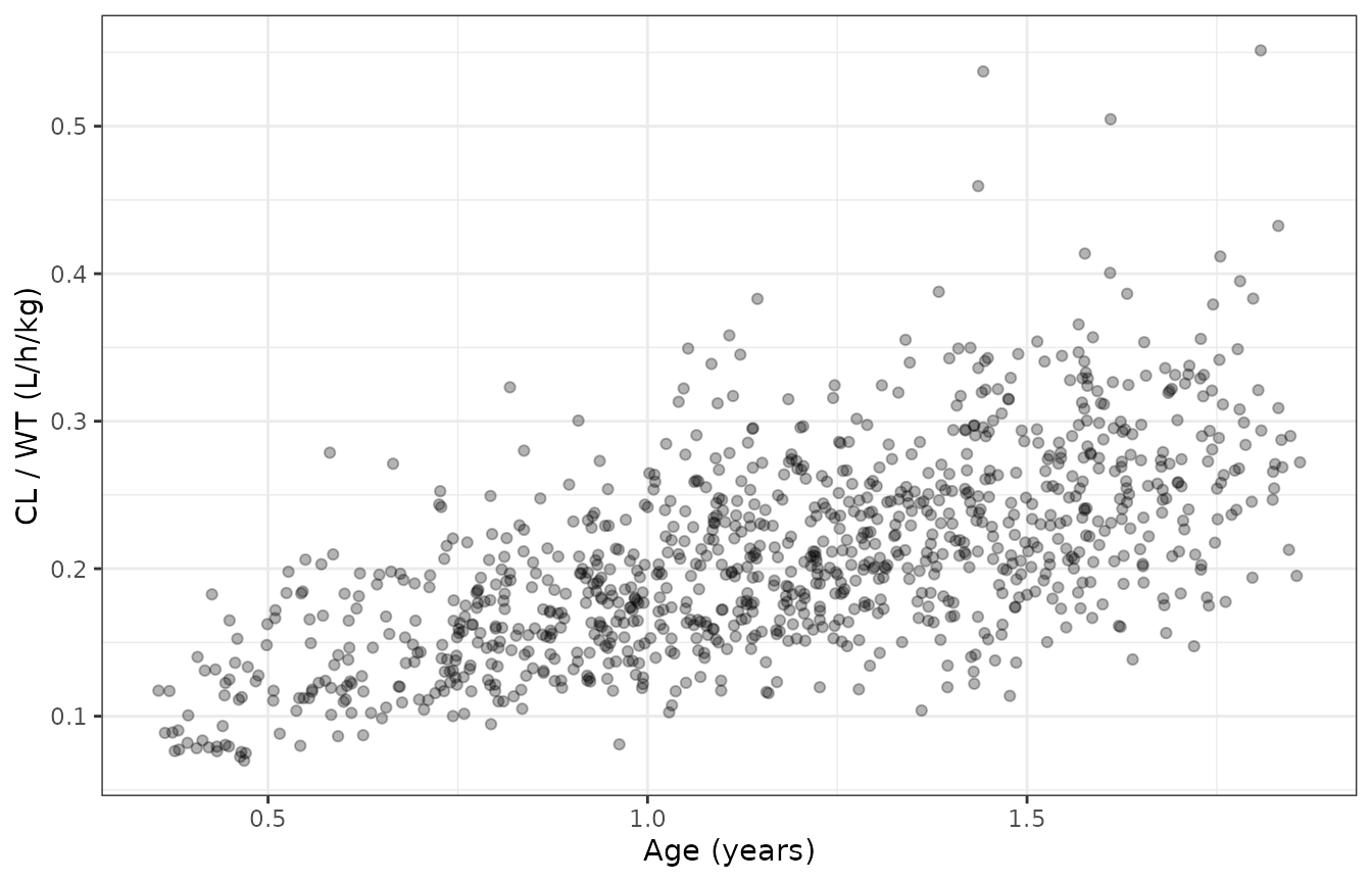

Individual weight-normalised clearance against age in the virtual cohort (compare Du 2021 Supplementary Figure S2).

The 1-2 year group matches the paper’s mean of 0.23 L/h/kg. The simulated infants aged <= 1 year have a higher mean clearance than the paper’s 0.11 L/h/kg, so the simulated contrast between the groups is smaller than the paper’s two-fold difference. The paper’s figure is a mean of individual estimates in a few infants (the group sizes are not reported), and those estimates also absorb any age effect beyond the fitted power term. The cohort here draws age and weight independently, so its youngest infants are not also its lightest; for comparison, the typical infant of 0.6 years and 8.5 kg has a model clearance of 0.14 L/h/kg.

Simulation at steady state

Three regimens are simulated for 5 days with 30-minute infusions: the prescribed 100 mg/kg/day q12h and the two recommended regimens, 50 mg/kg/day q8h and 75 mg/kg/day q6h. Because the half-life is about 1 hour, 5 days is effectively infinite dosing. The typical-value model (zeroRe()) is solved with each subject’s base-R random effects supplied as data columns.

regimens <- tibble(
  treatment = c("100 mg/kg/day q12h", "50 mg/kg/day q8h", "75 mg/kg/day q6h"),
  daily_mg_kg = c(100, 50, 75),
  tau = c(12, 8, 6)
)
t_inf <- 0.5
t_end <- 120
n_sim <- 200L

sim_cohort <- cohort |> filter(id <= n_sim)

make_events <- function(reg, subjects) {
  dose_times <- seq(0, t_end - reg$tau, by = reg$tau)
  last_dose <- max(dose_times)
  obs_times <- sort(unique(c(
    seq(0, last_dose, by = 2),
    last_dose + c(seq(0, t_inf, by = 0.05), seq(t_inf, reg$tau, by = 0.1))
  )))
  bind_rows(lapply(seq_len(nrow(subjects)), function(i) {
    s <- subjects[i, ]
    amt <- reg$daily_mg_kg * reg$tau / 24 * s$WT
    bind_rows(
      tibble(time = dose_times, evid = 1L, amt = amt, rate = amt / t_inf),
      tibble(time = obs_times, evid = 0L, amt = 0, rate = 0)
    ) |>
      mutate(
        id = s$id, cmt = "central", WT = s$WT, AGE = s$AGE,
        etalcl = s$etalcl, etalvc = s$etalvc,
        treatment = reg$treatment, last_dose = last_dose, tau = reg$tau
      )
  })) |>
    arrange(id, time, desc(evid))
}

mod_typ <- rxode2::zeroRe(mod_ui)

solve_regimen <- function(reg) {
  ev <- make_events(reg, sim_cohort)
  sim <- withCallingHandlers(
    rxode2::rxSolve(
      mod_typ,
      events = ev, keep = c("treatment", "WT"),
      rtol = 1e-10, atol = 1e-12, returnType = "data.frame"
    ),
    warning = function(w) {
      if (grepl("omega", conditionMessage(w))) invokeRestart("muffleWarning")
    }
  )
  sim$last_dose <- ev$last_dose[1]
  sim$tau <- reg$tau
  sim
}

sims <- bind_rows(lapply(seq_len(nrow(regimens)), function(i) {
  solve_regimen(regimens[i, ])
}))
#> ℹ omega/sigma items treated as zero: 'etalcl', 'etalvc'
#> ℹ omega/sigma items treated as zero: 'etalcl', 'etalvc'
#> ℹ omega/sigma items treated as zero: 'etalcl', 'etalvc'

The one-compartment infusion model has a closed-form steady-state solution. The ODE solve is checked against it for every subject and time point in the final dosing interval; both sides use the same individual parameters, so the difference is pure integration error.

css_closed_form <- function(dose, tau, tinf, cl, v, t) {
  k <- cl / v
  r <- dose / tinf
  c_end <- r / cl * (1 - exp(-k * tinf))
  current <- ifelse(
    t <= tinf,
    r / cl * (1 - exp(-k * t)),
    c_end * exp(-k * (t - tinf))
  )
  current + c_end * exp(-k * (t + tau - tinf)) / (1 - exp(-k * tau))
}

check_cf <- sims |>
  filter(time >= last_dose) |>
  left_join(
    regimens |> select(treatment, daily_mg_kg),
    by = "treatment"
  ) |>
  left_join(sim_cohort |> select(id, cl_i = cl, vc_i = vc), by = "id") |>
  mutate(
    cf = css_closed_form(
      daily_mg_kg * tau / 24 * WT, tau, t_inf, cl_i, vc_i, time - last_dose
    ),
    rel_err = Cc / cf - 1
  )

max(abs(check_cf$rel_err))
#> [1] 6.700366e-08
stopifnot(max(abs(check_cf$rel_err)) < 1e-5)

sims |>
  filter(time >= last_dose) |>
  mutate(tad = time - last_dose) |>
  group_by(treatment, tad) |>
  summarise(
    med = median(Cc), lo = quantile(Cc, 0.05), hi = quantile(Cc, 0.95),
    .groups = "drop"
  ) |>
  ggplot(aes(tad, med)) +
  geom_ribbon(aes(ymin = lo, ymax = hi), alpha = 0.25) +
  geom_line() +
  geom_hline(yintercept = c(0.5, 2) / 0.77, linetype = "dashed") +
  scale_y_log10() +
  facet_wrap(~treatment, scales = "free_x") +
  labs(x = "Time after dose (h)", y = "Cefathiamidine (mg/L)") +
  theme_bw()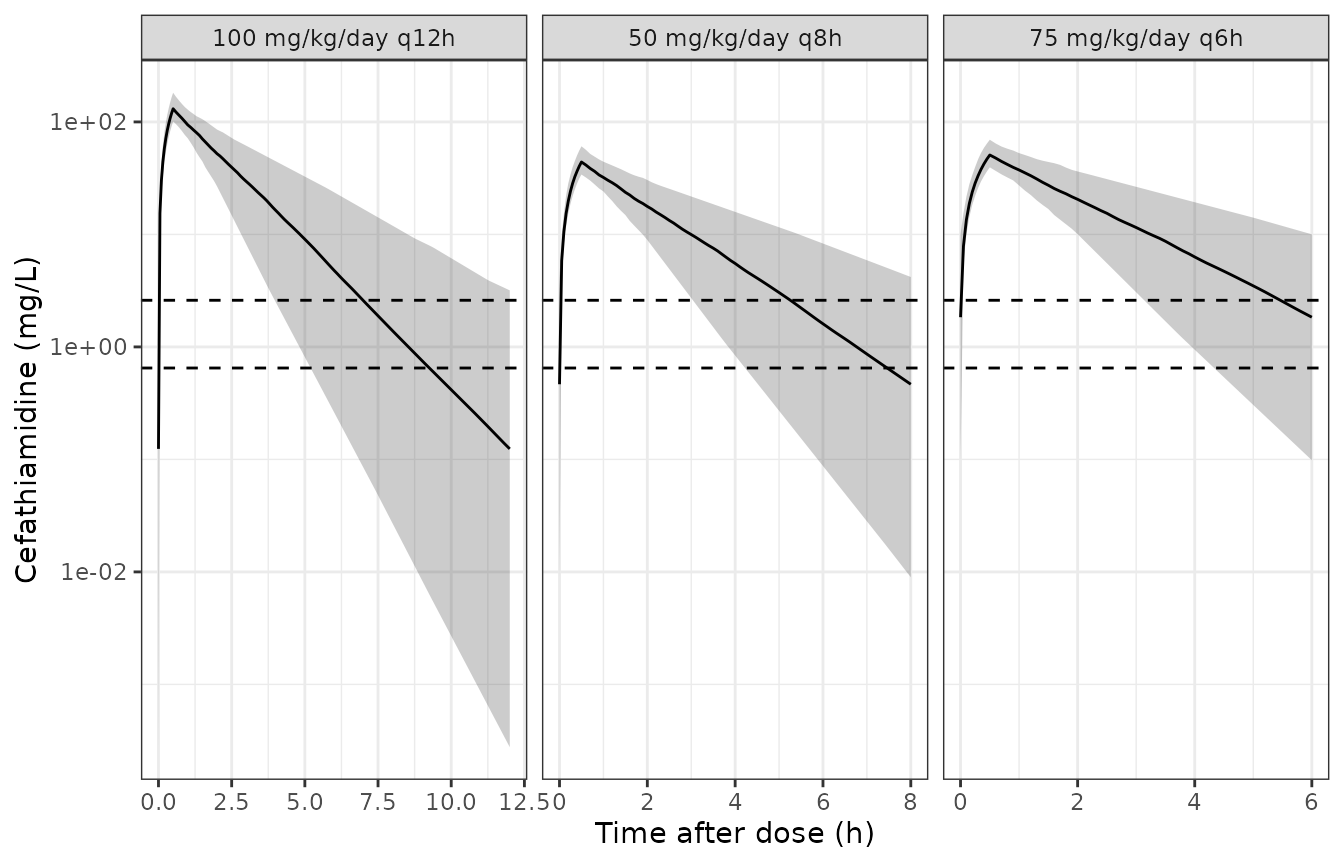

Steady-state total plasma concentrations over the final dosing interval (median and 5th-95th percentiles of 200 infants per regimen; between-subject variability only). The dashed lines mark the MICs 0.5 and 2 mg/L divided by the free fraction 0.77.

PKNCA validation

Steady-state NCA over the final dosing interval of each regimen, grouped by treatment. AUC0-24 is AUC over the interval multiplied by the number of doses per day.

conc_nca <- sims |>
  filter(time >= last_dose, !is.na(Cc)) |>
  select(id, time, Cc, treatment) |>
  as.data.frame()

dose_nca <- sims |>
  distinct(id, treatment, last_dose, tau) |>
  left_join(regimens |> select(treatment, daily_mg_kg), by = "treatment") |>
  left_join(sim_cohort |> select(id, WT), by = "id") |>
  transmute(
    id, treatment,
    time = last_dose, amt = daily_mg_kg * tau / 24 * WT
  ) |>
  as.data.frame()

conc_obj <- PKNCA::PKNCAconc(
  conc_nca, Cc ~ time | treatment + id,
  concu = "mg/L", timeu = "h"
)
dose_obj <- PKNCA::PKNCAdose(
  dose_nca, amt ~ time | treatment + id,
  doseu = "mg"
)
intervals <- regimens |>
  transmute(
    treatment,
    start = t_end - tau,
    end = t_end,
    cmax = TRUE, cmin = TRUE, tmax = TRUE, auclast = TRUE
  ) |>
  as.data.frame()

nca_res <- PKNCA::pk.nca(PKNCA::PKNCAdata(conc_obj, dose_obj, intervals = intervals))

nca_ind <- as.data.frame(nca_res) |>
  select(id, treatment, PPTESTCD, PPORRES) |>
  pivot_wider(names_from = PPTESTCD, values_from = PPORRES) |>
  left_join(regimens |> select(treatment, tau), by = "treatment") |>
  left_join(sim_cohort |> select(id, cl), by = "id") |>
  left_join(dose_nca |> select(id, treatment, amt), by = c("id", "treatment")) |>
  mutate(auc24 = auclast * 24 / tau, auc24_exact = amt * 24 / tau / cl)

nca_ind |>
  group_by(treatment) |>
  summarise(
    `Cmax median (mg/L)` = median(cmax),
    `Cmin median (mg/L)` = median(cmin),
    `AUC0-24 median (mg*h/L)` = median(auc24),
    `AUC0-24 5th` = quantile(auc24, 0.05),
    `AUC0-24 95th` = quantile(auc24, 0.95)
  ) |>
  knitr::kable(digits = 2)

treatment	Cmax median (mg/L)	Cmin median (mg/L)	AUC0-24 median (mg*h/L)	AUC0-24 5th	AUC0-24 95th
100 mg/kg/day q12h	130.99	0.12	506.73	309.31	904.83
50 mg/kg/day q8h	44.02	0.47	253.36	154.66	452.42
75 mg/kg/day q6h	50.81	1.84	380.05	231.98	678.62

# Trapezoidal AUC over a dense grid against the exact Dose/CL at steady state.
stopifnot(max(abs(nca_ind$auc24 / nca_ind$auc24_exact - 1)) < 0.01)

Comparison against published exposure

Du 2021 does not tabulate NCA parameters. The Results state that the individual steady-state AUC0-24 under the prescribed doses ranged from 296 to 1,152 mgh/L, and that the median weight-normalised clearance was 0.22 L/h/kg. For 100 mg/kg/day, AUC0-24 = daily dose / CL, so the median clearance implies a median AUC0-24 of 100 / 0.22 = 455 mgh/L; that derived value is the reference below.

sim_auc <- nca_ind |>
  filter(treatment == "100 mg/kg/day q12h") |>
  transmute(PPTESTCD = "auclast", PPORRES = auc24)
ref_auc <- data.frame(auclast = 100 / 0.22)

cmp <- nlmixr2lib::ncaComparisonTable(
  sim_auc, ref_auc,
  units = c(auclast = "mg*h/L"),
  tolerance_pct = 20
)
cmp[[1]] <- "AUC0-24 (100 mg/kg/day q12h)"
knitr::kable(cmp)

NCA parameter	Reference	Simulated	% diff
AUC0-24 (100 mg/kg/day q12h)	455	507	+11.5%

rng <- quantile(sim_auc$PPORRES, c(0.05, 0.95))
rng
#>       5%      95% 
#> 309.3101 904.8326

The simulated median AUC0-24 lies within 20% of the value implied by the paper’s median clearance, and the simulated 5th-95th percentile range overlaps the published individual range (296-1,152 mg*h/L; the published range also reflects the actual doses, 40-100 mg/kg per dose).

Probability of target attainment (Figure 2)

The paper’s target is 70% fT > MIC over the dosing interval, with a fixed unbound fraction of 0.77, evaluated in 1,000 simulated infants at MICs of 0.25, 0.5, 2 and 8 mg/L. Figure 2 is a bar chart; the values below are the ones quoted in the Results text.

The PTA is computed here from the closed-form steady-state profile of each of the 1,000 cohort members, evaluated on a 2,000-point grid over the interval. The calculation is repeated with the exponential residual error applied as a per-time-point probability, pnorm((log(C) - log(MIC)) / expSd); on a grid this dense the two versions agree to within half a percentage point (asserted below), so the paper’s choice on this point does not matter.

mic <- c(0.25, 0.5, 2, 8)
fu <- 0.77
exp_sd <- unname(mod_ui$theta["expSd"])
pta_regimens <- expand.grid(daily_mg_kg = c(50, 75, 100), tau = c(6, 8, 12))

pta <- bind_rows(lapply(seq_len(nrow(pta_regimens)), function(i) {
  reg <- pta_regimens[i, ]
  t_grid <- seq(0, reg$tau, length.out = 2001)[-2001]
  ft <- vapply(seq_len(n_cohort), function(j) {
    conc <- fu * css_closed_form(
      reg$daily_mg_kg * reg$tau / 24 * cohort$WT[j],
      reg$tau, t_inf, cohort$cl[j], cohort$vc[j], t_grid
    )
    c(
      vapply(mic, function(m) mean(conc > m), numeric(1)),
      # Expected fraction of the interval above MIC once the exponential
      # residual error is applied independently at each grid point.
      vapply(mic, function(m) mean(pnorm((log(conc) - log(m)) / exp_sd)), numeric(1))
    )
  }, numeric(2 * length(mic)))
  tibble(
    daily_mg_kg = reg$daily_mg_kg, tau = reg$tau, MIC = mic,
    pta_pct = 100 * rowMeans(ft[seq_along(mic), , drop = FALSE] >= 0.7),
    pta_resid_pct = 100 * rowMeans(ft[length(mic) + seq_along(mic), , drop = FALSE] >= 0.7)
  )
}))

max(abs(pta$pta_resid_pct - pta$pta_pct))
#> [1] 0.1
stopifnot(max(abs(pta$pta_resid_pct - pta$pta_pct)) < 0.5)

published <- tribble(
  ~daily_mg_kg, ~tau, ~MIC, ~paper_pct,
  100, 12, 0.25, 70.1,
  100, 12, 0.5, 58.3,
  100, 12, 2, 29.4,
  100, 12, 8, 8.3,
  50, 8, 0.5, 75.5,
  50, 8, 2, 36.3,
  75, 6, 2, 72.1,
  100, 6, 8, 30.8
)

pta_cmp <- published |>
  left_join(pta, by = c("daily_mg_kg", "tau", "MIC")) |>
  mutate(diff_pct_points = pta_pct - paper_pct)

pta_cmp |>
  mutate(
    regimen = sprintf("%g mg/kg/day q%gh", daily_mg_kg, tau),
    MIC = format(MIC, drop0trailing = TRUE)
  ) |>
  select(regimen, MIC, paper_pct, pta_pct, diff_pct_points) |>
  rename(
    Regimen = regimen,
    `MIC (mg/L)` = MIC,
    `Published PTA (%)` = paper_pct,
    `Simulated PTA (%)` = pta_pct,
    `Difference (points)` = diff_pct_points
  ) |>
  knitr::kable(digits = 1)

Regimen	MIC (mg/L)	Published PTA (%)	Simulated PTA (%)	Difference (points)
100 mg/kg/day q12h	0.25	70.1	71.6	1.5
100 mg/kg/day q12h	0.5	58.3	58.7	0.4
100 mg/kg/day q12h	2	29.4	30.1	0.7
100 mg/kg/day q12h	8	8.3	5.6	-2.7
50 mg/kg/day q8h	0.5	75.5	79.4	3.9
50 mg/kg/day q8h	2	36.3	39.0	2.7
75 mg/kg/day q6h	2	72.1	76.8	4.7
100 mg/kg/day q6h	8	30.8	31.7	0.9

# The cohort and random effects come from base R, so these values are
# reproducible on every platform; the bounds still leave room for the
# unpublished covariate distribution of the paper's simulation.
stopifnot(
  median(abs(pta_cmp$diff_pct_points)) < 4,
  all(abs(pta_cmp$diff_pct_points) < 8)
)

pta |>
  mutate(
    regimen = factor(sprintf("%g mg/kg/day q%gh", daily_mg_kg, tau)),
    MIC = factor(MIC)
  ) |>
  ggplot(aes(MIC, pta_pct)) +
  geom_col(fill = "grey70") +
  geom_point(
    data = published |>
      mutate(
        regimen = factor(sprintf("%g mg/kg/day q%gh", daily_mg_kg, tau)),
        MIC = factor(MIC)
      ),
    aes(MIC, paper_pct), colour = "black", size = 2
  ) +
  geom_hline(yintercept = 70, linetype = "dashed") +
  facet_wrap(~regimen) +
  labs(x = "MIC (mg/L)", y = "PTA (%)") +
  theme_bw()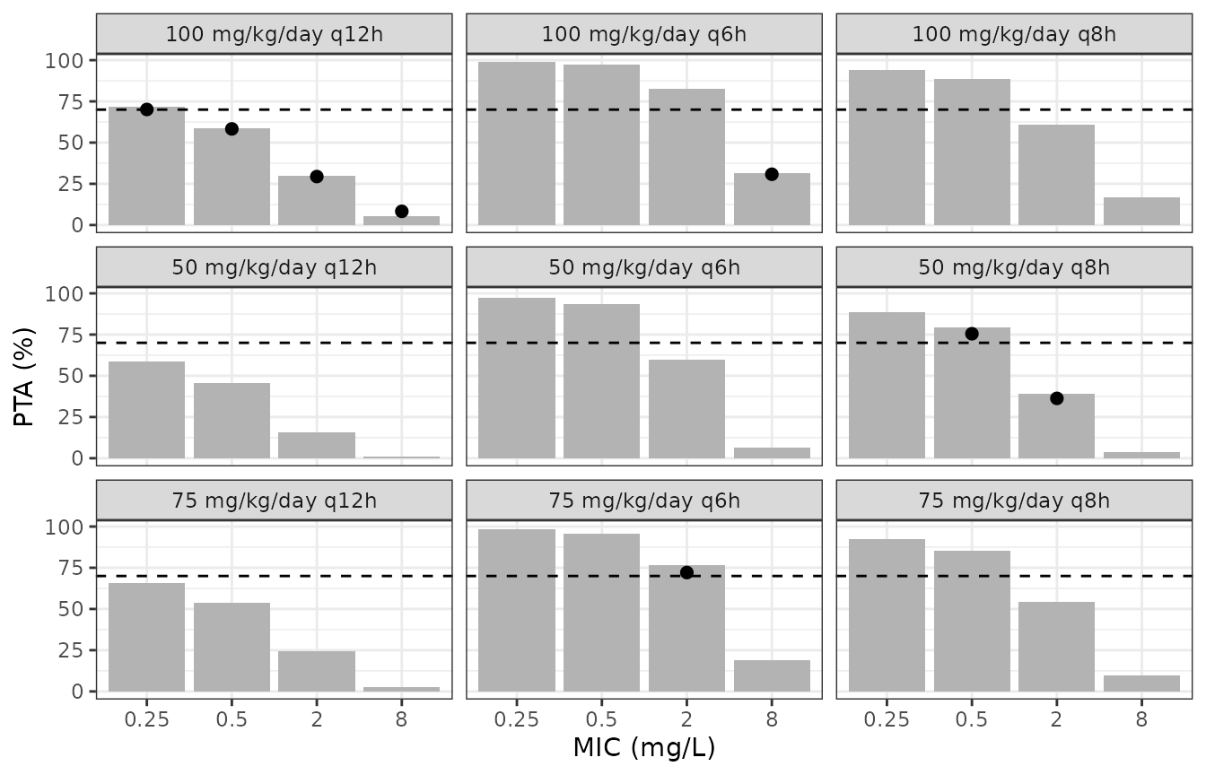

Simulated PTA for 70% fT > MIC by regimen and MIC (bars), with the values quoted in the Du 2021 Results text (points). Replicates Figure 2 of Du 2021.

The model reproduces the paper’s conclusions: the prescribed 100 mg/kg/day q12h regimen reaches 70% PTA only at MIC 0.25 mg/L, 50 mg/kg/day q8h does so at 0.5 mg/L, 75 mg/kg/day q6h at 2 mg/L, and even 100 mg/kg/day q6h falls far short at 8 mg/L.

Assumptions and deviations

• IIV and residual scale. Table 2 reports the IIV and residual error as percentages. They are converted as CV of a log-normal quantity: omega^2 = log(CV^2 + 1), and the log-scale residual SD sqrt(log(CV^2 + 1)). Reading them instead as omega = CV changes the variances by less than 4%.
• Weight range. The Results text gives the weight range as 8.0-12.5 kg and Table 1 as 8.00-13.00 kg. The table value is used for the metadata and the cohort.
• Virtual cohort. Weight and age were drawn independently from normal distributions with the Table 1 means and SDs, truncated to the observed ranges. The paper’s simulation resampled the 20 original infants, whose covariates are not published.
• PTA method. The paper does not say whether fT > MIC was evaluated at steady state or after the first dose, nor whether residual error was included. Steady state is used here; because the half-life is about 1 hour, accumulation is negligible for q8h and q12h and small for q6h. Residual error has no material effect in the dense-grid limit (see above).
• Infusion duration. 30 minutes for every simulated regimen, as in the study.