Nicotine pouch buccal-permeation PBPK (Salehi 2025)
Source:vignettes/articles/Salehi_2025_nicotine_pbpk.Rmd
Salehi_2025_nicotine_pbpk.RmdModel and source
Citation: Salehi A, Sarkar MA, Smith JH, Rostami AA. (2025). Physiologically Based Pharmacokinetic Modeling to Predict Nicotine Pharmacokinetics of Nicotine Pouches Under Naturalistic Use Conditions. J Clin Pharmacol 65(10):1297-1309. doi:10.1002/jcph.70038. PMCID PMC12484417. Correction added 2025-06-27 (final sentence of Methods; prose only, no parameter impact). Whole-body disposition structure and physiological / chemical parameters inherited from Rostami AA, Campbell JL, Pithawalla YB, et al. (2022) Sci Rep 12:1091, doi:10.1038/s41598-022-05108-y (with Author Correction, Sci Rep 12:2436, doi:10.1038/s41598-022-06693-8 – bibliography fix only).
Description: PBPK (whole-body, MCSim/deSolve). Nicotine, cotinine and nicotine glucuronide disposition in adults who use tobacco-free nicotine pouches, moist smokeless tobacco (MST) or intravenous nicotine (Salehi 2025). A buccal-cavity tissue permeation front-end solves Fick’s second law across the buccal epithelium as a 20-slab method-of-lines diffusion chain (buccal_slab1..buccal_slab20) with a released-nicotine flux boundary at the saliva interface and a perfect-sink boundary at the effective tissue depth; the sink-face flux is the blood uptake rate feeding the perfused buccal submucosa, and the balance of released nicotine that is swallowed enters the gut. The whole-body disposition model is inherited from Rostami 2022 with hepatic and urinary clearances reduced by 50 percent per Salehi 2025, and carries eleven flow-limited nicotine tissues plus a nicotine-driven heart-rate feedback on cardiac output, a five-tissue cotinine sub-model and a one-compartment nicotine-glucuronide sub-model. Deterministic typical-value model: the sources report no between-subject variability and no residual-error model. The inhalation (cigarette) route of the parent Rostami model is NOT implemented because its CFD-derived deposition fractions are unreported in every available source; see the vignette Errata.
Article: https://doi.org/10.1002/jcph.70038
Upstream framework paper (Rostami 2022): https://doi.org/10.1038/s41598-022-05108-y
Salehi 2025 couples a fit-for-purpose buccal-cavity (BC) tissue permeation model to the whole-body nicotine PBPK model of Rostami 2022, in order to predict nicotine exposure from tobacco-free nicotine pouches under naturalistic use conditions rather than the controlled single-use conditions of a clinical abuse-liability study. Two pouch products are studied: on! (referred to throughout as TP1, at 2 / 4 / 8 mg nicotine) and on! PLUS (TP2, at 6 / 9 / 12 mg), each compared against the subject’s own-brand moist smokeless tobacco (OBMST).
Population
The PBPK model is not fitted to individual-level data; it is regressed against cohort-mean plasma nicotine profiles. Those profiles come from randomized controlled single-use studies in adults who smoke cigarettes or use MST, with mean body weights of about 92 kg in the TP1 cohort and about 97 kg in the TP2 cohort (Salehi 2025, Figure 2 caption). The Rostami 2022 reference adult is 73.0 kg (Rostami 2022 Table 1).
Naturalistic use patterns come from a separate 6-week actual-use study: a median of about 6 pouches per day held in the mouth for about 12-13 min, and, for MST, 4-6 use occasions per day of 45-60 min (Salehi 2025, “AUS Data and Alternative Use Scenarios”).
str(ui$population)
#> List of 7
#>  $ species      : chr "human"
#>  $ age_range    : chr "adults who use tobacco products (21+ years)"
#>  $ weight_median: chr "92 kg (on! / TP1 cohort) and 97 kg (on! PLUS / TP2 cohort); Rostami 2022 reference adult 73.0 kg"
#>  $ disease_state: chr "healthy adults who smoke cigarettes or use moist smokeless tobacco"
#>  $ dose_range   : chr "on! nicotine pouches 2 / 4 / 8 mg (30 min controlled use); on! PLUS nicotine pouches 6 / 9 / 12 mg (45 min cont"| __truncated__
#>  $ regions      : chr "United States"
#>  $ notes        : chr "The PBPK model is not fitted to individual-level data. Clinical PK profiles used for the base-use-case regressi"| __truncated__
Source trace
Every ini() entry in
inst/modeldb/specificDrugs/Salehi_2025_nicotine_pbpk.R
carries an in-file comment naming its source location. The table below
collects them.
| Equation / parameter | Value | Source location |
|---|---|---|
Buccal tissue diffusion PDE, dC/dt = D d2C/dx2
|
n/a | Salehi 2025 Equation 1 |
| Flux boundary condition at the saliva interface | n/a | Salehi 2025 Equation 2 |
Perfect-sink boundary C(t, x = l) = 0
|
n/a | Salehi 2025 Methods, “Model Description” |
Blood uptake rate R_blood = sink-face flux |
n/a | Salehi 2025 Equation 5 |
| Linear (time-varying) tissue uptake for TP2 | n/a | Salehi 2025 Equation 6 |
Exponential release A0 (1 - exp(-k t))
|
n/a | Salehi 2025 Methods, “AUS Data and Alternative Use Scenarios” |
DBUC (nicotine diffusivity in BC) |
1.2e-5 cm^2/s | Salehi 2025 Results, “Tissue Permeation Model Parameters” |
LBUC (effective BC tissue thickness) |
0.175 cm | Salehi 2025 Results, “Tissue Permeation Model Parameters” |
KA1 (GI uptake rate constant) |
0.8 /h | Salehi 2025 Results, “GI Tract Uptake Rate Constant” |
FTISM / FTISE (tissue uptake
fractions) |
product-specific | Salehi 2025 Table 2 |
KREL (product release rate constant) |
product-specific | Salehi 2025 Table 2 (MST) and Methods “Clinical Data” (pouch extraction fractions) |
| MST buccal uptake fraction | 0.25 | Salehi 2025 Methods, “Parameters” (about 25% of released nicotine taken up) |
| Hepatic / urinary clearances, halved |
CLMC 1.35, CLKC 0.21, CLLMC
0.07, CLKMC 0.0125 |
Rostami 2022 Table 2, halved per Salehi 2025 Methods (“reduced by 50%”) |
FA (oral bioavailability) |
0.67 | Rostami 2022 Table 2 |
FNC (fraction to cotinine) |
0.80 | Rostami 2022 Table 2 |
FNG, VGDC, GCLC (glucuronide
sub-model) |
0.10, 1.0, 0.1 | Salehi 2025 supplementary MCSim listing |
| Tissue volumes and blood flows | see ini()
|
Rostami 2022 Table 1 |
| Surface areas and epithelial widths | see ini()
|
Rostami 2022 Table 1 |
| Partition coefficients (nicotine, cotinine) | see ini()
|
Rostami 2022 Table 2 |
Tissue binding BMLURC, BMHRC,
KBLU, KBH
|
0.00235, 0.00427, 0, 0 | Salehi 2025 supplementary MCSim listing |
Heart-rate feedback SPD, KANT,
CANT50
|
933.66, 1.6617, 0.0152 | Rostami 2022 Table 2 |
| Cotinine / glucuronide molecular weights | 178, 338 | Salehi 2025 supplementary MCSim listing (hard-coded literals) |
Simulation setup
The model is deterministic: neither Salehi 2025 nor Rostami 2022
reports between-subject variability or a residual-error model, so there
are no eta terms to simulate and every arm below is a
single typical-value profile.
Nicotine release is first-order loss from the depot
compartment (the product in the mouth). Because a used pouch or pinch is
discarded rather than fully extracted, the end of each use
occasion is encoded as a replacement event (evid = 5,
amt = 0) that zeroes depot; any nicotine still
unreleased leaves with the product. Multiple use occasions therefore
compose correctly, which is what Scenario III needs.
# Release rate constant implied by an extraction fraction over a use duration:
# A0 (1 - exp(-k t_use)) = frac * A0.
krel_from_extraction <- function(frac, tuse) -log(1 - frac) / tuse

# Salehi 2025 Methods, "Clinical Data": about 61% of TP1 8 mg extracted over
# 30 min, and 67-72% of TP2 extracted over 45 min (70% adopted; see Errata).
krel_tp1 <- krel_from_extraction(0.61, 0.5)
krel_tp2 <- krel_from_extraction(0.70, 0.75)

# One row per simulated arm. a0 = nicotine content of one product unit (mg);
# MST assumes about 10 mg nicotine per g of unused product (Salehi 2025
# Methods, "Parameters"), so a 2 g pinch is 20 mg.
base_arms <- tibble::tribble(
  ~arm,         ~product, ~a0, ~tuse, ~krel,    ~ftism, ~ftise, ~fswal, ~wt,
  "TP1 2 mg",   "TP1",      2,  0.50, krel_tp1,   0.50,   0.50,      1,  92,
  "TP1 4 mg",   "TP1",      4,  0.50, krel_tp1,   0.51,   0.51,      1,  92,
  "TP1 8 mg",   "TP1",      8,  0.50, krel_tp1,   0.46,   0.46,      1,  92,
  "TP2 6 mg",   "TP2",      6,  0.75, krel_tp2,   0.38,   0.22,      1,  97,
  "TP2 9 mg",   "TP2",      9,  0.75, krel_tp2,   0.35,   0.20,      1,  97,
  "TP2 12 mg",  "TP2",     12,  0.75, krel_tp2,   0.35,   0.15,      1,  97,
  "OBMST 2 g",  "OBMST",   20,  0.50, 0.73,       0.25,   0.25,      0,  92,
  "OBMST 4 g",  "OBMST",   40,  0.75, 0.55,       0.25,   0.25,      0,  97
)

knitr::kable(
  base_arms |>
    dplyr::mutate(krel = round(krel, 4)) |>
    dplyr::rename(
      "Arm" = arm, "Product" = product, "Nicotine content (mg)" = a0,
      "Use duration (h)" = tuse, "Release k (1/h)" = krel,
      "Mean uptake fraction" = ftism, "End uptake fraction" = ftise,
      "Swallowed fraction" = fswal, "Body weight (kg)" = wt
    ),
  caption = "Base use cases. Adjusted parameters are from Salehi 2025 Table 2."
)| Arm | Product | Nicotine content (mg) | Use duration (h) | Release k (1/h) | Mean uptake fraction | End uptake fraction | Swallowed fraction | Body weight (kg) |
|---|---|---|---|---|---|---|---|---|
| TP1 2 mg | TP1 | 2 | 0.50 | 1.8832 | 0.50 | 0.50 | 1 | 92 |
| TP1 4 mg | TP1 | 4 | 0.50 | 1.8832 | 0.51 | 0.51 | 1 | 92 |
| TP1 8 mg | TP1 | 8 | 0.50 | 1.8832 | 0.46 | 0.46 | 1 | 92 |
| TP2 6 mg | TP2 | 6 | 0.75 | 1.6053 | 0.38 | 0.22 | 1 | 97 |
| TP2 9 mg | TP2 | 9 | 0.75 | 1.6053 | 0.35 | 0.20 | 1 | 97 |
| TP2 12 mg | TP2 | 12 | 0.75 | 1.6053 | 0.35 | 0.15 | 1 | 97 |
| OBMST 2 g | OBMST | 20 | 0.50 | 0.7300 | 0.25 | 0.25 | 0 | 92 |
| OBMST 4 g | OBMST | 40 | 0.75 | 0.5500 | 0.25 | 0.25 | 0 | 97 |
mod <- readModelDb("Salehi_2025_nicotine_pbpk")

# Solve one arm: `n_use` product-use occasions spaced `interval` hours apart.
# Product-specific quantities live in ini(); body weight is a data covariate.
solve_arm <- function(arm, a0, tuse, krel, ftism, ftise, fswal, wt,
                      n_use = 1L, interval = 0, tmax = 3.5, dt = 1 / 60) {
  m <- mod |>
    rxode2::ini(KREL = krel, TUSE = tuse, FTISM = ftism,
                FTISE = ftise, FSWAL = fswal)
  starts <- (seq_len(n_use) - 1L) * interval
  ev <- rxode2::et(amt = a0, cmt = "depot", time = starts) |>
    # end of each use occasion: the product is removed and discarded
    rxode2::et(amt = 0, cmt = "depot", time = starts + tuse, evid = 5) |>
    # observations on an ODE state, never on an algebraic observable
    rxode2::et(seq(0, tmax, by = dt), cmt = "a_venous")
  rxode2::rxSolve(m, ev, params = c(WT = wt),
                  atol = 1e-10, rtol = 1e-8) |>
    as.data.frame() |>
    dplyr::filter(!duplicated(time)) |>
    dplyr::mutate(arm = arm)
}

# Row-wise apply: each column of `df` becomes a named argument of `f`.
apply_rows <- function(df, f, ...) {
  do.call(
    mapply,
    c(list(FUN = f, SIMPLIFY = FALSE, MoreArgs = list(...)), as.list(df))
  )
}

solve_arms <- function(arms, ...) {
  arms |>
    dplyr::select(arm, a0, tuse, krel, ftism, ftise, fswal, wt) |>
    apply_rows(solve_arm, ...) |>
    dplyr::bind_rows() |>
    dplyr::left_join(arms |> dplyr::select(arm, product), by = "arm") |>
    dplyr::mutate(arm = factor(arm, levels = arms$arm))
}
Replicate published figures
Figure 2 – base use cases
# Replicates Figure 2 of Salehi 2025: single use of TP1 (30 min), TP2 (45 min)
# and the subject's OBMST product.
sim_base <- solve_arms(base_arms)
#> ℹ change initial estimate of `KREL` to `1.88321707971689`
#> ℹ change initial estimate of `TUSE` to `0.5`
#> ℹ change initial estimate of `FTISM` to `0.5`
#> ℹ change initial estimate of `FTISE` to `0.5`
#> ℹ change initial estimate of `FSWAL` to `1`
#> ℹ change initial estimate of `KREL` to `1.88321707971689`
#> ℹ change initial estimate of `TUSE` to `0.5`
#> ℹ change initial estimate of `FTISM` to `0.51`
#> ℹ change initial estimate of `FTISE` to `0.51`
#> ℹ change initial estimate of `FSWAL` to `1`
#> ℹ change initial estimate of `KREL` to `1.88321707971689`
#> ℹ change initial estimate of `TUSE` to `0.5`
#> ℹ change initial estimate of `FTISM` to `0.46`
#> ℹ change initial estimate of `FTISE` to `0.46`
#> ℹ change initial estimate of `FSWAL` to `1`
#> ℹ change initial estimate of `KREL` to `1.60529707243458`
#> ℹ change initial estimate of `TUSE` to `0.75`
#> ℹ change initial estimate of `FTISM` to `0.38`
#> ℹ change initial estimate of `FTISE` to `0.22`
#> ℹ change initial estimate of `FSWAL` to `1`
#> ℹ change initial estimate of `KREL` to `1.60529707243458`
#> ℹ change initial estimate of `TUSE` to `0.75`
#> ℹ change initial estimate of `FTISM` to `0.35`
#> ℹ change initial estimate of `FTISE` to `0.2`
#> ℹ change initial estimate of `FSWAL` to `1`
#> ℹ change initial estimate of `KREL` to `1.60529707243458`
#> ℹ change initial estimate of `TUSE` to `0.75`
#> ℹ change initial estimate of `FTISM` to `0.35`
#> ℹ change initial estimate of `FTISE` to `0.15`
#> ℹ change initial estimate of `FSWAL` to `1`
#> ℹ change initial estimate of `KREL` to `0.73`
#> ℹ change initial estimate of `TUSE` to `0.5`
#> ℹ change initial estimate of `FTISM` to `0.25`
#> ℹ change initial estimate of `FTISE` to `0.25`
#> ℹ change initial estimate of `FSWAL` to `0`
#> ℹ change initial estimate of `KREL` to `0.55`
#> ℹ change initial estimate of `TUSE` to `0.75`
#> ℹ change initial estimate of `FTISM` to `0.25`
#> ℹ change initial estimate of `FTISE` to `0.25`
#> ℹ change initial estimate of `FSWAL` to `0`

ggplot(sim_base, aes(time * 60, Cc, colour = arm)) +
  geom_line(linewidth = 0.7) +
  facet_wrap(~product, scales = "free_y") +
  labs(x = "Time (min)", y = "Venous plasma nicotine (ng/mL)",
       colour = NULL,
       title = "Figure 2 -- base use cases",
       caption = "Replicates Figure 2 of Salehi 2025 (panels a-c).") +
  theme(legend.position = "bottom")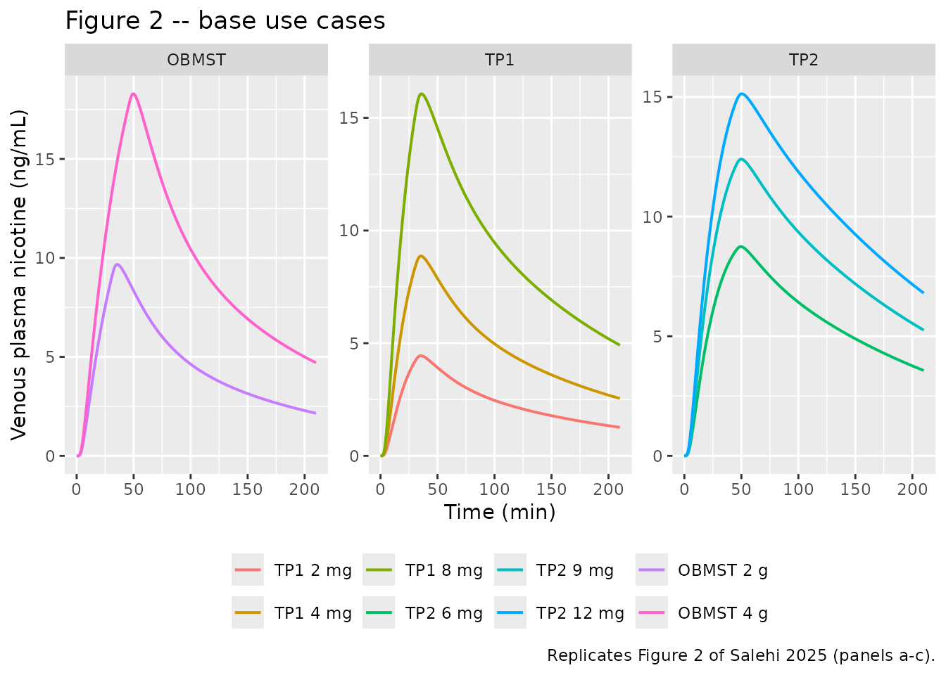
Figure S3 – intravenous validation
The intravenous arm exercises the whole-body disposition model with no buccal component at all, and reproduces the qualitative signature of Figure S3: arterial concentrations run well above venous during the infusion and converge to them afterwards.
# Replicates Figure S3 of Salehi 2025: 2 ug/kg/min over 30 min in an 85 kg
# adult (Gourlay & Benowitz 1997). A placeholder amt = 0 depot record is
# required so tad(depot) is defined -- see the model file's section 4 comment.
iv_dose <- 2e-3 * 85 * 30  # mg delivered over 30 min
ev_iv <- rxode2::et(amt = 0, cmt = "depot", time = 0) |>
  rxode2::et(amt = iv_dose, dur = 0.5, cmt = "a_arterial") |>
  rxode2::et(seq(0, 6, by = 1 / 120), cmt = "a_venous")

sim_iv <- rxode2::rxSolve(mod, ev_iv, params = c(WT = 85),
                          atol = 1e-10, rtol = 1e-8) |>
  as.data.frame() |>
  dplyr::filter(!duplicated(time))

sim_iv |>
  dplyr::select(time, Venous = Cc, Arterial = Cart) |>
  tidyr::pivot_longer(-time, names_to = "Site", values_to = "conc") |>
  ggplot(aes(time, conc, colour = Site)) +
  geom_line(linewidth = 0.7) +
  geom_vline(xintercept = 0.5, linetype = "dashed", colour = "grey50") +
  labs(x = "Time (h)", y = "Plasma nicotine (ng/mL)",
       title = "Figure S3 -- 2 ug/kg/min intravenous nicotine over 30 min",
       caption = paste("Replicates Figure S3 of Salehi 2025.",
                       "Dashed line = end of infusion."))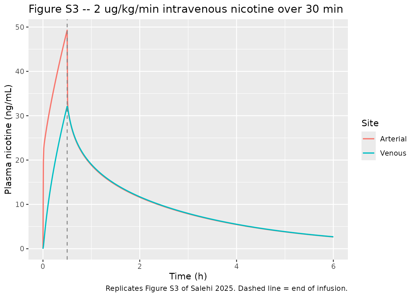
# The arterial > venous separation during infusion, and convergence after it,
# is the qualitative claim of Figure S3. Assert it rather than eyeball it.
during <- dplyr::filter(sim_iv, time > 0.05, time <= 0.5)
after  <- dplyr::filter(sim_iv, time >= 2)
stopifnot(
  nrow(during) > 0, nrow(after) > 0,
  all(during$Cart > during$Cc),
  max(abs(after$Cart - after$Cc) / after$Cc) < 0.05
)
c(
  venous_peak_ng_mL   = round(max(sim_iv$Cc), 2),
  arterial_peak_ng_mL = round(max(sim_iv$Cart), 2),
  cotinine_6h_ng_mL   = round(dplyr::last(sim_iv$Cc_cot), 2)
)
#>   venous_peak_ng_mL arterial_peak_ng_mL   cotinine_6h_ng_mL
#>               32.14               49.29               34.95
Figures 3 and 4 – Scenario I and Scenario II
Scenario I uses the median time-in-mouth from the actual-use study; Scenario II uses a conservative 90th-percentile time-in-mouth (Salehi 2025 Table 1). Only the use duration changes – the product release constant and the tissue uptake fractions are held at their base-use-case values, as the paper does.
scenario_i <- base_arms |>
  dplyr::mutate(tuse = dplyr::case_when(
    product %in% c("TP1", "TP2") ~ 15 / 60,
    product == "OBMST"           ~ 45 / 60
  ))

# Table 1: TP1 25 min; TP2 6 mg 30 min, TP2 9 and 12 mg 40 min; OBMST 75 min.
scenario_ii <- base_arms |>
  dplyr::mutate(tuse = dplyr::case_when(
    product == "TP1"     ~ 25 / 60,
    arm == "TP2 6 mg"    ~ 30 / 60,
    product == "TP2"     ~ 40 / 60,
    product == "OBMST"   ~ 75 / 60
  ))

sim_i  <- solve_arms(scenario_i,  tmax = 4)
#> ℹ change initial estimate of `KREL` to `1.88321707971689`
#> ℹ change initial estimate of `TUSE` to `0.25`
#> ℹ change initial estimate of `FTISM` to `0.5`
#> ℹ change initial estimate of `FTISE` to `0.5`
#> ℹ change initial estimate of `FSWAL` to `1`
#> ℹ change initial estimate of `KREL` to `1.88321707971689`
#> ℹ change initial estimate of `TUSE` to `0.25`
#> ℹ change initial estimate of `FTISM` to `0.51`
#> ℹ change initial estimate of `FTISE` to `0.51`
#> ℹ change initial estimate of `FSWAL` to `1`
#> ℹ change initial estimate of `KREL` to `1.88321707971689`
#> ℹ change initial estimate of `TUSE` to `0.25`
#> ℹ change initial estimate of `FTISM` to `0.46`
#> ℹ change initial estimate of `FTISE` to `0.46`
#> ℹ change initial estimate of `FSWAL` to `1`
#> ℹ change initial estimate of `KREL` to `1.60529707243458`
#> ℹ change initial estimate of `TUSE` to `0.25`
#> ℹ change initial estimate of `FTISM` to `0.38`
#> ℹ change initial estimate of `FTISE` to `0.22`
#> ℹ change initial estimate of `FSWAL` to `1`
#> ℹ change initial estimate of `KREL` to `1.60529707243458`
#> ℹ change initial estimate of `TUSE` to `0.25`
#> ℹ change initial estimate of `FTISM` to `0.35`
#> ℹ change initial estimate of `FTISE` to `0.2`
#> ℹ change initial estimate of `FSWAL` to `1`
#> ℹ change initial estimate of `KREL` to `1.60529707243458`
#> ℹ change initial estimate of `TUSE` to `0.25`
#> ℹ change initial estimate of `FTISM` to `0.35`
#> ℹ change initial estimate of `FTISE` to `0.15`
#> ℹ change initial estimate of `FSWAL` to `1`
#> ℹ change initial estimate of `KREL` to `0.73`
#> ℹ change initial estimate of `TUSE` to `0.75`
#> ℹ change initial estimate of `FTISM` to `0.25`
#> ℹ change initial estimate of `FTISE` to `0.25`
#> ℹ change initial estimate of `FSWAL` to `0`
#> ℹ change initial estimate of `KREL` to `0.55`
#> ℹ change initial estimate of `TUSE` to `0.75`
#> ℹ change initial estimate of `FTISM` to `0.25`
#> ℹ change initial estimate of `FTISE` to `0.25`
#> ℹ change initial estimate of `FSWAL` to `0`
sim_ii <- solve_arms(scenario_ii, tmax = 4)
#> ℹ change initial estimate of `KREL` to `1.88321707971689`
#> ℹ change initial estimate of `TUSE` to `0.416666666666667`
#> ℹ change initial estimate of `FTISM` to `0.5`
#> ℹ change initial estimate of `FTISE` to `0.5`
#> ℹ change initial estimate of `FSWAL` to `1`
#> ℹ change initial estimate of `KREL` to `1.88321707971689`
#> ℹ change initial estimate of `TUSE` to `0.416666666666667`
#> ℹ change initial estimate of `FTISM` to `0.51`
#> ℹ change initial estimate of `FTISE` to `0.51`
#> ℹ change initial estimate of `FSWAL` to `1`
#> ℹ change initial estimate of `KREL` to `1.88321707971689`
#> ℹ change initial estimate of `TUSE` to `0.416666666666667`
#> ℹ change initial estimate of `FTISM` to `0.46`
#> ℹ change initial estimate of `FTISE` to `0.46`
#> ℹ change initial estimate of `FSWAL` to `1`
#> ℹ change initial estimate of `KREL` to `1.60529707243458`
#> ℹ change initial estimate of `TUSE` to `0.5`
#> ℹ change initial estimate of `FTISM` to `0.38`
#> ℹ change initial estimate of `FTISE` to `0.22`
#> ℹ change initial estimate of `FSWAL` to `1`
#> ℹ change initial estimate of `KREL` to `1.60529707243458`
#> ℹ change initial estimate of `TUSE` to `0.666666666666667`
#> ℹ change initial estimate of `FTISM` to `0.35`
#> ℹ change initial estimate of `FTISE` to `0.2`
#> ℹ change initial estimate of `FSWAL` to `1`
#> ℹ change initial estimate of `KREL` to `1.60529707243458`
#> ℹ change initial estimate of `TUSE` to `0.666666666666667`
#> ℹ change initial estimate of `FTISM` to `0.35`
#> ℹ change initial estimate of `FTISE` to `0.15`
#> ℹ change initial estimate of `FSWAL` to `1`
#> ℹ change initial estimate of `KREL` to `0.73`
#> ℹ change initial estimate of `TUSE` to `1.25`
#> ℹ change initial estimate of `FTISM` to `0.25`
#> ℹ change initial estimate of `FTISE` to `0.25`
#> ℹ change initial estimate of `FSWAL` to `0`
#> ℹ change initial estimate of `KREL` to `0.55`
#> ℹ change initial estimate of `TUSE` to `1.25`
#> ℹ change initial estimate of `FTISM` to `0.25`
#> ℹ change initial estimate of `FTISE` to `0.25`
#> ℹ change initial estimate of `FSWAL` to `0`

dplyr::bind_rows(
  sim_i  |> dplyr::mutate(scenario = "Scenario I (median use)"),
  sim_ii |> dplyr::mutate(scenario = "Scenario II (90th percentile use)")
) |>
  ggplot(aes(time * 60, Cc, colour = arm)) +
  geom_line(linewidth = 0.7) +
  facet_grid(scenario ~ product, scales = "free_y") +
  labs(x = "Time (min)", y = "Venous plasma nicotine (ng/mL)", colour = NULL,
       title = "Figures 3 and 4 -- alternative single-use scenarios",
       caption = "Replicates Figures 3 and 4 of Salehi 2025 (panels a-c).") +
  theme(legend.position = "bottom")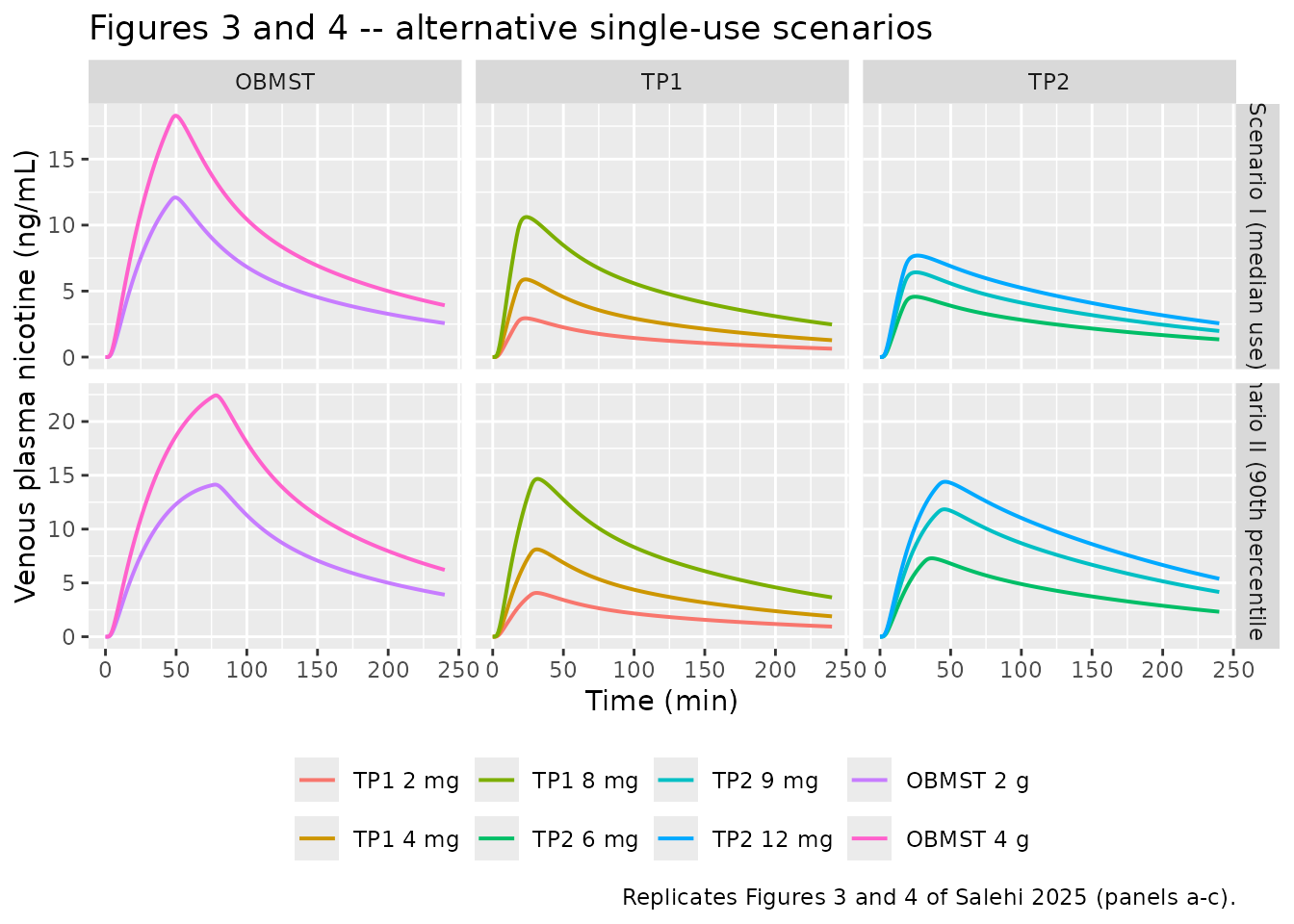
Figure 5 – Scenario III, multiple use occasions over a day
Six pouches or five MST occasions spread evenly over a 16 h waking period (Salehi 2025 Table 1).
scenario_iii <- base_arms |>
  dplyr::mutate(
    tuse     = dplyr::if_else(product == "OBMST", 45 / 60, 15 / 60),
    n_use    = dplyr::if_else(product == "OBMST", 5L, 6L),
    interval = 16 / n_use
  )

sim_iii <- scenario_iii |>
  dplyr::select(arm, a0, tuse, krel, ftism, ftise, fswal, wt, n_use, interval) |>
  apply_rows(solve_arm, tmax = 24, dt = 1 / 30) |>
  dplyr::bind_rows() |>
  dplyr::left_join(base_arms |> dplyr::select(arm, product), by = "arm") |>
  dplyr::mutate(arm = factor(arm, levels = base_arms$arm)) |>
  dplyr::group_by(arm) |>
  dplyr::mutate(
    cumauc = c(0, cumsum(diff(time) * (head(Cc, -1) + tail(Cc, -1)) / 2))
  ) |>
  dplyr::ungroup()
#> ℹ change initial estimate of `KREL` to `1.88321707971689`
#> ℹ change initial estimate of `TUSE` to `0.25`
#> ℹ change initial estimate of `FTISM` to `0.5`
#> ℹ change initial estimate of `FTISE` to `0.5`
#> ℹ change initial estimate of `FSWAL` to `1`
#> ℹ change initial estimate of `KREL` to `1.88321707971689`
#> ℹ change initial estimate of `TUSE` to `0.25`
#> ℹ change initial estimate of `FTISM` to `0.51`
#> ℹ change initial estimate of `FTISE` to `0.51`
#> ℹ change initial estimate of `FSWAL` to `1`
#> ℹ change initial estimate of `KREL` to `1.88321707971689`
#> ℹ change initial estimate of `TUSE` to `0.25`
#> ℹ change initial estimate of `FTISM` to `0.46`
#> ℹ change initial estimate of `FTISE` to `0.46`
#> ℹ change initial estimate of `FSWAL` to `1`
#> ℹ change initial estimate of `KREL` to `1.60529707243458`
#> ℹ change initial estimate of `TUSE` to `0.25`
#> ℹ change initial estimate of `FTISM` to `0.38`
#> ℹ change initial estimate of `FTISE` to `0.22`
#> ℹ change initial estimate of `FSWAL` to `1`
#> ℹ change initial estimate of `KREL` to `1.60529707243458`
#> ℹ change initial estimate of `TUSE` to `0.25`
#> ℹ change initial estimate of `FTISM` to `0.35`
#> ℹ change initial estimate of `FTISE` to `0.2`
#> ℹ change initial estimate of `FSWAL` to `1`
#> ℹ change initial estimate of `KREL` to `1.60529707243458`
#> ℹ change initial estimate of `TUSE` to `0.25`
#> ℹ change initial estimate of `FTISM` to `0.35`
#> ℹ change initial estimate of `FTISE` to `0.15`
#> ℹ change initial estimate of `FSWAL` to `1`
#> ℹ change initial estimate of `KREL` to `0.73`
#> ℹ change initial estimate of `TUSE` to `0.75`
#> ℹ change initial estimate of `FTISM` to `0.25`
#> ℹ change initial estimate of `FTISE` to `0.25`
#> ℹ change initial estimate of `FSWAL` to `0`
#> ℹ change initial estimate of `KREL` to `0.55`
#> ℹ change initial estimate of `TUSE` to `0.75`
#> ℹ change initial estimate of `FTISM` to `0.25`
#> ℹ change initial estimate of `FTISE` to `0.25`
#> ℹ change initial estimate of `FSWAL` to `0`

sim_iii |>
  dplyr::select(time, arm, product,
                `Plasma nicotine (ng/mL)` = Cc,
                `Cumulative AUC (ng*h/mL)` = cumauc) |>
  tidyr::pivot_longer(c(-time, -arm, -product)) |>
  ggplot(aes(time, value, colour = arm)) +
  geom_line(linewidth = 0.6) +
  facet_wrap(~name, scales = "free_y", ncol = 1) +
  labs(x = "Time (h)", y = NULL, colour = NULL,
       title = "Figure 5 -- Scenario III, multiple use occasions",
       caption = "Replicates Figure 5 of Salehi 2025.") +
  theme(legend.position = "bottom")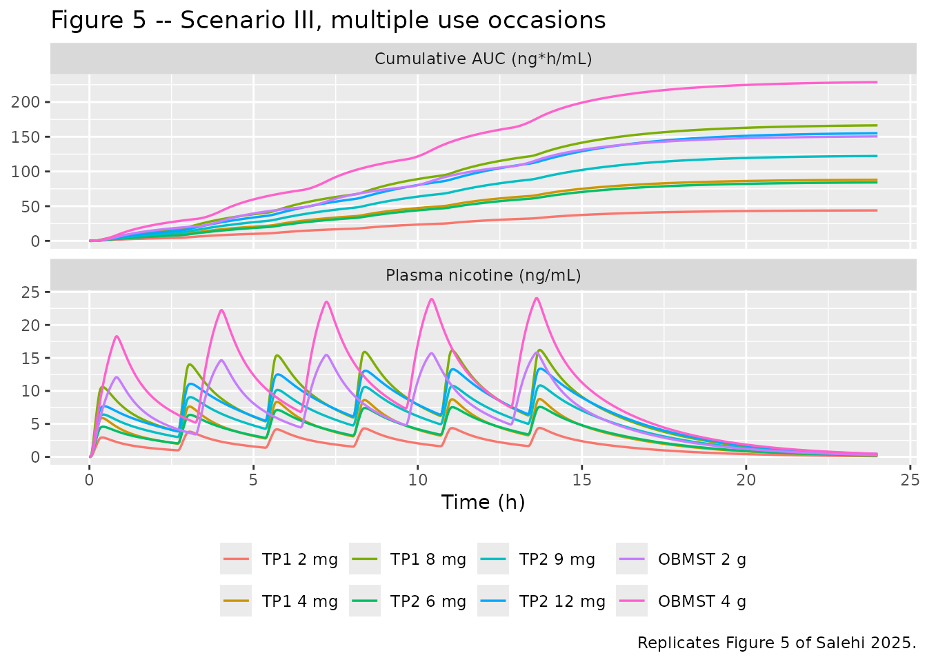
# The paper's central claim for Scenario III: cumulative daily nicotine
# exposure from either pouch is not higher than from OBMST use.
day_auc <- sim_iii |>
  dplyr::group_by(arm, product) |>
  dplyr::summarise(auc24 = max(cumauc), .groups = "drop")

stopifnot(
  max(day_auc$auc24[day_auc$product %in% c("TP1", "TP2")]) <
    max(day_auc$auc24[day_auc$product == "OBMST"])
)

day_auc |>
  dplyr::mutate(auc24 = round(auc24, 1)) |>
  dplyr::rename("Arm" = arm, "Product" = product,
                "Cumulative AUC0-24h (ng*h/mL)" = auc24) |>
knitr::kable(caption = "Scenario III cumulative 24 h nicotine exposure.")| Arm | Product | Cumulative AUC0-24h (ng*h/mL) |
|---|---|---|
| TP1 2 mg | TP1 | 43.9 |
| TP1 4 mg | TP1 | 88.1 |
| TP1 8 mg | TP1 | 166.4 |
| TP2 6 mg | TP2 | 84.2 |
| TP2 9 mg | TP2 | 122.4 |
| TP2 12 mg | TP2 | 155.1 |
| OBMST 2 g | OBMST | 150.5 |
| OBMST 4 g | OBMST | 228.6 |
PKNCA validation
Table 2 of Salehi 2025 reports AUC over 0-180 min (footnote b), so the NCA interval below is 0-3 h rather than 0-infinity.
sim_nca <- sim_base |>
  dplyr::filter(!is.na(Cc)) |>
  dplyr::mutate(id = as.integer(arm)) |>
  dplyr::select(id, time, Cc, arm)

# Guarantee a time = 0 row per arm; pre-dose nicotine is 0 by construction.
sim_nca <- dplyr::bind_rows(
  sim_nca,
  sim_nca |> dplyr::distinct(id, arm) |> dplyr::mutate(time = 0, Cc = 0)
) |>
  dplyr::distinct(id, arm, time, .keep_all = TRUE) |>
  dplyr::arrange(id, time)

conc_obj <- PKNCA::PKNCAconc(sim_nca, Cc ~ time | arm + id)

dose_df <- base_arms |>
  dplyr::mutate(id = dplyr::row_number(), time = 0) |>
  dplyr::select(id, time, amt = a0, arm)
dose_obj <- PKNCA::PKNCAdose(dose_df, amt ~ time | arm + id)

intervals <- data.frame(
  start = 0, end = 3,
  cmax = TRUE, tmax = TRUE, auclast = TRUE
)

nca_res <- PKNCA::pk.nca(PKNCA::PKNCAdata(conc_obj, dose_obj,
                                          intervals = intervals))
Comparison against the paper’s own predictions
Table 2 of Salehi 2025 reports the AUC its own implementation predicts for each base use case. Reproducing that column is the implementation-fidelity check for this extraction.
published_predicted <- tibble::tribble(
  ~arm,        ~auclast,
  "TP1 2 mg",       7.3,
  "TP1 4 mg",      13.9,
  "TP1 8 mg",      27.1,
  "TP2 6 mg",      20.0,
  "TP2 9 mg",      30.5,
  "TP2 12 mg",     38.8,
  "OBMST 2 g",     15.0,
  "OBMST 4 g",     30.6
)

cmp <- nlmixr2lib::ncaComparisonTable(
  simulated     = nca_res,
  reference     = published_predicted,
  by            = "arm",
  params        = "auclast",
  units         = c(auclast = "ng*h/mL"),
  tolerance_pct = 20
)

knitr::kable(
  cmp,
  caption = paste("Simulated AUC(0-3 h) against the model-predicted AUC",
                  "column of Salehi 2025 Table 2.",
                  "* differs from reference by >20%."),
  digits = 2
)| NCA parameter | arm | Reference | Simulated | % diff |
|---|---|---|---|---|
| AUClast (ng*h/mL) | TP1 2 mg | 7.3 | 7.58 | +3.9% |
| AUClast (ng*h/mL) | TP1 4 mg | 13.9 | 15.3 | +9.7% |
| AUClast (ng*h/mL) | TP1 8 mg | 27.1 | 28.5 | +5.3% |
| AUClast (ng*h/mL) | TP2 6 mg | 20 | 17.6 | -11.9% |
| AUClast (ng*h/mL) | TP2 9 mg | 30.5 | 25.4 | -16.7% |
| AUClast (ng*h/mL) | TP2 12 mg | 38.8 | 31.9 | -17.8% |
| AUClast (ng*h/mL) | OBMST 2 g | 15 | 14.9 | -0.8% |
| AUClast (ng*h/mL) | OBMST 4 g | 30.6 | 30.3 | -1.0% |
Comparison against the observed clinical AUC
observed <- tibble::tribble(
  ~arm,        ~obs, ~lo,  ~hi,
  "TP1 2 mg",   7.1,  6.1,  8.3,
  "TP1 4 mg",  13.5, 11.6, 15.7,
  "TP1 8 mg",  24.2, 20.8, 28.0,
  "TP2 6 mg",  19.6, 18.5, 20.8,
  "TP2 9 mg",  29.7, 28.0, 31.5,
  "TP2 12 mg", 37.1, 35.4, 40.3,
  "OBMST 2 g", 16.6, 14.4, 19.1,
  "OBMST 4 g", 31.6, 29.2, 34.2
)

nca_wide <- as.data.frame(nca_res) |>
  dplyr::select(arm, PPTESTCD, PPORRES) |>
  tidyr::pivot_wider(names_from = PPTESTCD, values_from = PPORRES)

obs_tab <- observed |>
  dplyr::left_join(nca_wide, by = "arm") |>
  dplyr::mutate(
    within_ci = auclast >= lo & auclast <= hi,
    pct_diff  = 100 * (auclast - obs) / obs
  )

obs_tab |>
  dplyr::transmute(
    Arm                            = arm,
    `Cmax (ng/mL)`                 = round(cmax, 2),
    `Tmax (min)`                   = round(tmax * 60, 0),
    `Simulated AUC0-3h (ng*h/mL)`  = round(auclast, 1),
    `Observed AUC0-3h (90% CI)`    = sprintf("%.1f (%.1f-%.1f)", obs, lo, hi),
    `% difference`                 = round(pct_diff, 1),
    `Within observed 90% CI`       = ifelse(within_ci, "yes", "no")
  ) |>
  knitr::kable(
    caption = paste("Simulated NCA against the observed clinical AUC of",
                    "Salehi 2025 Table 2. Cmax and Tmax are simulated only;",
                    "the paper reports them graphically, not numerically.")
)| Arm | Cmax (ng/mL) | Tmax (min) | Simulated AUC0-3h (ng*h/mL) | Observed AUC0-3h (90% CI) | % difference | Within observed 90% CI |
|---|---|---|---|---|---|---|
| TP1 2 mg | 4.45 | 35 | 7.6 | 7.1 (6.1-8.3) | 6.8 | yes |
| TP1 4 mg | 8.87 | 35 | 15.3 | 13.5 (11.6-15.7) | 13.0 | yes |
| TP1 8 mg | 16.07 | 36 | 28.5 | 24.2 (20.8-28.0) | 17.9 | no |
| TP2 6 mg | 8.75 | 50 | 17.6 | 19.6 (18.5-20.8) | -10.1 | no |
| TP2 9 mg | 12.40 | 50 | 25.4 | 29.7 (28.0-31.5) | -14.4 | no |
| TP2 12 mg | 15.13 | 50 | 31.9 | 37.1 (35.4-40.3) | -14.1 | no |
| OBMST 2 g | 9.67 | 36 | 14.9 | 16.6 (14.4-19.1) | -10.4 | yes |
| OBMST 4 g | 18.29 | 50 | 30.3 | 31.6 (29.2-34.2) | -4.2 | yes |
# Guard the fidelity claim made in the narrative below, and make sure the
# lookup actually had rows to test (a check that cannot go red is not a check).
fidelity <- obs_tab |>
  dplyr::left_join(published_predicted |> dplyr::rename(paper_pred = auclast),
                   by = "arm") |>
  dplyr::mutate(pct_vs_paper = 100 * (auclast - paper_pred) / paper_pred)
stopifnot(nrow(fidelity) == 8L, !anyNA(fidelity$pct_vs_paper))

constant_arms <- c("TP1 2 mg", "TP1 4 mg", "TP1 8 mg", "OBMST 2 g", "OBMST 4 g")
constant_uptake <- dplyr::filter(fidelity, arm %in% constant_arms)
stopifnot(nrow(constant_uptake) == 5L,
          max(abs(constant_uptake$pct_vs_paper)) < 10)

c(
  constant_uptake_mean_abs_pct = round(mean(abs(constant_uptake$pct_vs_paper)), 1),
  constant_uptake_max_abs_pct  = round(max(abs(constant_uptake$pct_vs_paper)), 1)
)
#> constant_uptake_mean_abs_pct  constant_uptake_max_abs_pct
#>                          4.2                          9.7
Across the five constant-tissue-uptake arms (all three TP1 nicotine levels and both MST pinch weights) this implementation reproduces the paper’s own predicted AUC to a mean absolute difference of about 4%, with a maximum of under 10%. The two MST arms are a genuinely independent check: they use a different adjusted parameter (a fitted release rate constant rather than a tissue uptake fraction) and a different gastrointestinal assumption (the product is expectorated, so nothing is swallowed), and both land within about 1%.
The three TP2 arms sit 12-18% below the paper’s predictions. That gap is discussed under Errata below; it is a consequence of an internal inconsistency in the paper’s Equation 6, not of a transcription error, and nothing has been tuned to close it.
Assumptions and deviations
Errata and known inconsistencies in the source
Equation 6 is internally inconsistent, and is implemented exactly as printed. The TP2 linear tissue-uptake model reads
f_tissue(t) = ((f_e - f_bar) / 2) * (t / t_use) + (f_e + f_bar) / 2At t = t_use this evaluates to exactly f_e,
which satisfies Table 2 footnote d (“tissue uptake fraction at
45 min”). But its time-average over the use period is
(3 f_e + f_bar) / 4, not f_bar, which
contradicts footnote c (“mean tissue uptake fraction”) and the
sentence immediately below the equation, which states that
f_bar “denote[s] the average tissue uptake fraction”. The
equation and the prose cannot both be right.
Because the model exposes the two endpoints of the printed straight
line as FTISM and FTISE, any linear
reading can be simulated by remapping them. Writing the intended line as
f(t) = a + b (t / t_use), the model reproduces it with
FTISM = a - b and FTISE = a + b. The four
candidate readings are compared below against the paper’s TP2 AUCs of
20.0 / 30.5 / 38.8 – computed live rather than transcribed, so the table
cannot go stale.
tp2 <- tibble::tribble(
  ~arm,        ~a0, ~fbar, ~fe,   ~ref,
  "TP2 6 mg",    6,  0.38, 0.22,  20.0,
  "TP2 9 mg",    9,  0.35, 0.20,  30.5,
  "TP2 12 mg",  12,  0.35, 0.15,  38.8
)

# Each reading expressed as intercept `a` and slope `b` of f(t) = a + b*(t/tuse).
readings <- list(
  "A -- Equation 6 exactly as printed"        = function(fbar, fe) c((fe + fbar) / 2, (fe - fbar) / 2),
  "B -- ramp from f_bar down to f_e"          = function(fbar, fe) c(fbar, fe - fbar),
  "C -- endpoint f_e AND time-average f_bar"  = function(fbar, fe) c(2 * fbar - fe, 2 * (fe - fbar)),
  "D -- constant f_bar, ignoring f_e"         = function(fbar, fe) c(fbar, 0)
)

auc03 <- function(a0, a, b) {
  d <- solve_arm("x", a0 = a0, tuse = 0.75, krel = krel_tp2,
                 ftism = a - b, ftise = a + b, fswal = 1, wt = 97)
  d <- dplyr::filter(d, time <= 3 + 1e-9)
  sum(diff(d$time) * (head(d$Cc, -1) + tail(d$Cc, -1)) / 2)
}

eq6 <- lapply(names(readings), function(nm) {
  ab   <- Map(readings[[nm]], tp2$fbar, tp2$fe)
  aucs <- mapply(function(a0, p) auc03(a0, p[1], p[2]), tp2$a0, ab)
  tibble::tibble(
    Reading  = nm,
    `f(0)`   = paste(sprintf("%.2f", vapply(ab, `[`, numeric(1), 1)), collapse = " / "),
    AUCs     = paste(sprintf("%.1f", aucs), collapse = " / "),
    `% diff` = paste(sprintf("%+.0f%%", 100 * (aucs - tp2$ref) / tp2$ref),
                     collapse = " / ")
  )
}) |>
  dplyr::bind_rows()
#> ℹ change initial estimate of `KREL` to `1.60529707243458`
#> ℹ change initial estimate of `TUSE` to `0.75`
#> ℹ change initial estimate of `FTISM` to `0.38`
#> ℹ change initial estimate of `FTISE` to `0.22`
#> ℹ change initial estimate of `FSWAL` to `1`
#> ℹ change initial estimate of `KREL` to `1.60529707243458`
#> ℹ change initial estimate of `TUSE` to `0.75`
#> ℹ change initial estimate of `FTISM` to `0.35`
#> ℹ change initial estimate of `FTISE` to `0.2`
#> ℹ change initial estimate of `FSWAL` to `1`
#> ℹ change initial estimate of `KREL` to `1.60529707243458`
#> ℹ change initial estimate of `TUSE` to `0.75`
#> ℹ change initial estimate of `FTISM` to `0.35`
#> ℹ change initial estimate of `FTISE` to `0.15`
#> ℹ change initial estimate of `FSWAL` to `1`
#> ℹ change initial estimate of `KREL` to `1.60529707243458`
#> ℹ change initial estimate of `TUSE` to `0.75`
#> ℹ change initial estimate of `FTISM` to `0.54`
#> ℹ change initial estimate of `FTISE` to `0.22`
#> ℹ change initial estimate of `FSWAL` to `1`
#> ℹ change initial estimate of `KREL` to `1.60529707243458`
#> ℹ change initial estimate of `TUSE` to `0.75`
#> ℹ change initial estimate of `FTISM` to `0.5`
#> ℹ change initial estimate of `FTISE` to `0.2`
#> ℹ change initial estimate of `FSWAL` to `1`
#> ℹ change initial estimate of `KREL` to `1.60529707243458`
#> ℹ change initial estimate of `TUSE` to `0.75`
#> ℹ change initial estimate of `FTISM` to `0.55`
#> ℹ change initial estimate of `FTISE` to `0.15`
#> ℹ change initial estimate of `FSWAL` to `1`
#> ℹ change initial estimate of `KREL` to `1.60529707243458`
#> ℹ change initial estimate of `TUSE` to `0.75`
#> ℹ change initial estimate of `FTISM` to `0.86`
#> ℹ change initial estimate of `FTISE` to `0.22`
#> ℹ change initial estimate of `FSWAL` to `1`
#> ℹ change initial estimate of `KREL` to `1.60529707243458`
#> ℹ change initial estimate of `TUSE` to `0.75`
#> ℹ change initial estimate of `FTISM` to `0.8`
#> ℹ change initial estimate of `FTISE` to `0.2`
#> ℹ change initial estimate of `FSWAL` to `1`
#> ℹ change initial estimate of `KREL` to `1.60529707243458`
#> ℹ change initial estimate of `TUSE` to `0.75`
#> ℹ change initial estimate of `FTISM` to `0.95`
#> ℹ change initial estimate of `FTISE` to `0.15`
#> ℹ change initial estimate of `FSWAL` to `1`
#> ℹ change initial estimate of `KREL` to `1.60529707243458`
#> ℹ change initial estimate of `TUSE` to `0.75`
#> ℹ change initial estimate of `FTISM` to `0.38`
#> ℹ change initial estimate of `FTISE` to `0.38`
#> ℹ change initial estimate of `FSWAL` to `1`
#> ℹ change initial estimate of `KREL` to `1.60529707243458`
#> ℹ change initial estimate of `TUSE` to `0.75`
#> ℹ change initial estimate of `FTISM` to `0.35`
#> ℹ change initial estimate of `FTISE` to `0.35`
#> ℹ change initial estimate of `FSWAL` to `1`
#> ℹ change initial estimate of `KREL` to `1.60529707243458`
#> ℹ change initial estimate of `TUSE` to `0.75`
#> ℹ change initial estimate of `FTISM` to `0.35`
#> ℹ change initial estimate of `FTISE` to `0.35`
#> ℹ change initial estimate of `FSWAL` to `1`

# Guard the narrative claims below: the printed reading must under-predict, and
# every reading's f(0) must be a valid fraction for the impossibility claim to
# be decidable at all.
stopifnot(nrow(eq6) == 4L, all(grepl("^-", strsplit(eq6$`% diff`[1], " / ")[[1]])))

knitr::kable(eq6, caption = paste(
  "Candidate readings of Equation 6 for TP2 6 / 9 / 12 mg,",
  "against the paper's predicted AUCs of 20.0 / 30.5 / 38.8 ng*h/mL."
))| Reading | f(0) | AUCs | % diff |
|---|---|---|---|
| A – Equation 6 exactly as printed | 0.30 / 0.28 / 0.25 | 17.6 / 25.4 / 31.9 | -12% / -17% / -18% |
| B – ramp from f_bar down to f_e | 0.38 / 0.35 / 0.35 | 19.0 / 27.3 / 35.2 | -5% / -10% / -9% |
| C – endpoint f_e AND time-average f_bar | 0.54 / 0.50 / 0.55 | 21.7 / 31.1 / 41.9 | +9% / +2% / +8% |
| D – constant f_bar, ignoring f_e | 0.38 / 0.35 / 0.35 | 20.8 / 29.8 / 39.6 | +4% / -2% / +2% |
Reading A, exactly as printed, is the one implemented. That is the standing convention when a paper’s prose and its printed equation disagree, and reading A is the only candidate that is actually written down in the paper. It is, however, the worst-fitting of the four, and this vignette does not pretend otherwise: the honest summary is that the printed equation under-predicts the paper’s own TP2 AUCs by 12-18%, while readings C and D – neither of which appears in the paper – reproduce them to within roughly 10% and 4% respectively.
Reading C deserves particular note because it is the unique linear
function that satisfies both footnotes simultaneously
(endpoint f_e, time-average f_bar), and its
f(0) values of about 0.5-0.55 are perfectly valid uptake
fractions. It is therefore a live possibility for what the authors
intended, not something that can be dismissed. Reading D fits best of
all, but the paper states plainly that “the longer use duration of TP2,
45 min, required the model to allow for variable tissue uptake” and that
“the F-test … indicated that the linear form proved a better choice over
a constant tissue uptake”, so a constant uptake fraction contradicts the
paper’s own model-selection argument.
Nothing has been tuned to close the gap. A user who
prefers a different reading can obtain it without editing the model, by
setting FTISM and FTISE to the
a - b / a + b remapping shown in the chunk
above. For reference, the same code reproduces all five constant-uptake
arms – where f_e equals f_bar and every
reading collapses to the same constant – to about 4%.
CLM is assigned twice in the published MCSim
listing. The code reads CLM = CLMC*pow(BW,0.75)
and then, four lines later, CLM = CLMC*BW. MCSim’s
generated C keeps the last assignment, so hepatic metabolic clearance is
linear in body weight while every other clearance is allometric. The
duplication is present identically in both Salehi 2025 and Rostami 2022.
Both readings were tested against Table 2: as-coded (linear) gives about
4% mean absolute error, the allometric reading about 40%. The as-coded
reading is implemented.
Fat uses a multiplication where every other tissue
divides. The listing has CVF = CF*PF against
CVM = CM/PM, CVL = CL/PL, and so on. Fat is
25.8% of body weight, so this is not cosmetic. As-coded gives about 4%
mean absolute error against Table 2 and the “corrected”
CF/PF gives about 5%, so the as-coded reading is
implemented.
FNC conflicts between the table and the
code. Rostami 2022 Table 2 gives 0.80 (citing Robinson et al.);
both papers’ MCSim listings carry 0.72. The published table value is
adopted. This is immaterial to nicotine itself – FNC only
splits already-metabolized nicotine between cotinine and other routes
and does not enter nicotine’s own kinetics – but it does shift the
cotinine sub-model by about 10%.
Scope
The inhalation (cigarette) comparator arm is not
implemented. The parent Rostami model reaches the respiratory
tract through CFD-derived per-compartment deposition fractions
(DEPFRACBUC / DEPFRACCA /
DEPFRACTA / DEPFRACPU) and respiratory
mass-transfer coefficients. Every one of these is a 0
placeholder in both papers’ published code; Rostami 2022
tabulates none of them and attributes them to Adrian 2006, Asgharian
2011 and Corley 2012, none of which is open access, and the deposition
fractions are in any case outputs of an unpublished CFD model. The main
text (“90% of the inhaled dose deposited in the upper respiratory
tract”) and Figures S1/S2 (“95% … deposited in lower respiratory tract”)
also disagree, and neither gives the four-way split the code requires.
This is a reporting gap that no further source can close, so the
cigarette arm is omitted rather than guessed at. Its one fitted
parameter (a nicotine yield of 2.0 mg/cigarette, Table 2) is reported
and is recorded here for completeness.
The nicotine mouth-spray validation of Figure 1 is out of
scope. It is the one case that takes the Equation 3 branch
(flux back out of the tissue is non-negligible), which needs an
instantaneous saliva volume V_Sal. No baseline saliva
volume is reported in any available source. For the pouches and for MST
the paper takes the R_rel(t > t_use) = 0 branch, where
the GI input reduces analytically to
(1 - f_tissue(t)) * R_rel(t) and no saliva volume is
needed. Omitting Figure 1 costs only a validation of D and
l, both of which are taken as given here.
The parallel perfused-lung and nasal compartments of the
parent model are dropped. Their blood flow fractions
QLNGC and QNC are absent from Rostami 2022
Table 1 – whose flow fractions already sum to 1.0015 without them – and
are 0 in the published code, which comments the parallel
lung compartment as “only used for lung concentration (blood exchange is
cfd)”. Both compartments are therefore mathematically inert. This is the
code’s own declared value, not a substitution.
Numerical choices
The buccal diffusion PDE is solved by a 20-slab method of
lines. rxode2 solves ODEs only, so Equation 1 is discretised
into 20 equal slabs (buccal_slab1 …
buccal_slab20) with a mass-conserving finite-volume scheme
and a half-cell correction at the perfect-sink face. The slab count is a
numerical choice, not a property of the paper, so it is reported here:
AUC is identical to four decimal places from 10 slabs up to 80, and 20
slabs puts Cmax within 0.03% of an 80-slab solution. The chain cannot be
collapsed to a single well-mixed compartment – the diffusion time across
the tissue, l^2 / D = 0.71 h, is comparable to the use
duration, so the transient spatial profile is load-bearing.
Unreported values
-
No between-subject variability and no residual-error
model are reported in any available source, so none is encoded.
The model is deterministic typical-value only. Salehi 2025 does explore
inter-individual variability in the extent of nicotine release
by simulation (Figure S10), but reports no variance parameters that
could be carried into
ini(). - TP2 release fraction per nicotine level. Reported only as a range, 67-72% (SD 28-32%), described as spanning “different nicotine levels and flavors” and not resolved per level. 70% is used for all three levels, consistent with the paper’s own finding that release is not affected by nicotine level. Sensitivity across the full 67-72% range moves TP2 AUC by only about 3%, so this is not the source of the Equation 6 gap.
-
Nicotine molecular weight is declared as a
0placeholder in the published MCSim listing (whose.ininput files were never published) and is set here to the physical constant 162.23 g/mol. Cotinine and glucuronide use the listing’s own hard-coded literals of 178 and 338 g/mol. - Body weights for the alternative-use scenarios are not restated by the paper; the study-matched weights from the Figure 2 caption are carried forward (92 kg for TP1 and 2 g MST, 97 kg for TP2 and 4 g MST). Using the Rostami reference 73 kg instead degrades the MST base cases from about 1% to +22 / +28%, which confirms the study-matched reading.