Semaglutide (Overgaard 2019)
Source:vignettes/articles/Overgaard_2019_semaglutide.Rmd
Overgaard_2019_semaglutide.RmdModel and source
- Citation: Overgaard RV, Delff PH, Petri KCC, Anderson TW, Flint A, Ingwersen SH. Population pharmacokinetics of semaglutide for type 2 diabetes. Diabetes Therapy. 2019;10(2):649-662.
- DOI: https://doi.org/10.1007/s13300-019-0581-y
- Description: Two-compartment population PK model with first-order subcutaneous absorption and first-order elimination, fit jointly to nine clinical pharmacology trials (subcutaneous and intravenous administration; 353 subjects; 10,573 concentrations).
Population
The pooled clinical pharmacology cohort (Overgaard 2019 Table 3, two-compartment column) comprised 353 subjects: 277 normoglycaemic and 76 with type 2 diabetes (T2D). Body weight ranged from 51.9 to 121.2 kg (mean 81.9 kg, SD 15.1); age 19-70 years (mean 44.6 years); 36% female; 92.6% White, 4.5% Asian, 0.8% Black, 2.0% Other/missing. A 25-subject hepatic-impairment subgroup was included. Subcutaneous semaglutide was given at 0.25, 0.5, 1.0, or 1.5 mg once weekly; one trial (trial 7) administered 0.25 mg as a single intravenous bolus. Drug-product strengths were 1, 1.34, 3, and 10 mg/mL; the marketed strength is 1.34 mg/mL.
The reference subject for the final-model parameter estimates is a healthy, white, non-Hispanic female aged <= 65 years with body weight 85 kg, abdomen injection site, and 1.34 mg/mL drug product (Overgaard 2019, Methods page 654). All subsequent simulations in this vignette therefore use 85 kg + abdomen + 1.34 mg/mL as the reference.
The same population summary is available programmatically via
readModelDb("Overgaard_2019_semaglutide")$meta$population
after devtools::load_all().
Source trace
Per-parameter origins are recorded as in-file comments next to each
ini() entry in
inst/modeldb/specificDrugs/Overgaard_2019_semaglutide.R.
The table below collects them in one place.
| Equation / parameter | Value | Source location |
|---|---|---|
| Two-compartment SC + IV ODE structure | n/a | Overgaard 2019 Methods page 653 (“Model Description”) |
lka = log(0.0253) (1/h, 1.34 mg/mL, healthy) |
0.0253 | Table 4, row “Absorption rate constant (ka)” |
lcl = log(0.0348) (L/h, 85 kg, healthy) |
0.0348 | Table 4, row “Clearance (CL)” |
lvc = log(3.59) (L, 85 kg) |
3.59 | Table 4, row “Central volume (Vc)” |
lq = log(0.304) (L/h, 85 kg) |
0.304 | Table 4, row “Intercompartmental clearance (Q)” |
lvp = log(4.10) (L, 85 kg) |
4.10 | Table 4, row “Peripheral volume (Vp)” |
lfdepot = log(0.847) (abdomen, 1.34 mg/mL) |
0.847 | Table 4, row “Absolute bioavailability (F)” |
e_wt_cl_q (BW exponent on CL and Q) |
1.01 | Table 4, row “Body weight effect on CL and Q” |
e_wt_vc_vp (BW exponent on Vc and Vp) |
0.923 | Table 4, row “Body weight effect on Vc and Vp” |
e_diab_cl (T2D multiplier on CL) |
1.12 | Table 4, row “T2D effect on CL” |
e_diab_ka (T2D multiplier on ka) |
0.544 | Table 4, row “T2D effect on ka” |
| IIV CL = 15.2% CV -> omega^2 = log(1 + 0.152^2) = 0.022840 | 0.022840 | Table 4, IIV (% CV) column for CL |
| IIV Vc = 15.4% CV -> omega^2 = log(1 + 0.154^2) = 0.023438 | 0.023438 | Table 4, IIV (% CV) column for Vc |
| Cov(eta_CL, eta_Vc) | 0.0172 | Table 4 footnote (“A covariance of 0.0172 was found between CL and Vc”) |
| IIV ka = 37.9% CV -> omega^2 = log(1 + 0.379^2) = 0.133844 | 0.133844 | Table 4, IIV (% CV) column for ka |
propSd (additive on log scale ~ proportional in
linear) |
0.103 | Table 4, row “Residual error” + Methods page 654 (“residual error model was additive for log-transformed observations”) |
Covariate-effect parameterization (Methods page 653, equations on page 653-654):
| Effect | Functional form | Implementation in model()
|
|---|---|---|
| Body weight on CL | (WT/85)^1.01 | (WT / 85)^e_wt_cl_q |
| Body weight on Q | (WT/85)^1.01 (shared exponent) | (WT / 85)^e_wt_cl_q |
| Body weight on Vc | (WT/85)^0.923 | (WT / 85)^e_wt_vc_vp |
| Body weight on Vp | (WT/85)^0.923 (shared exponent) | (WT / 85)^e_wt_vc_vp |
| T2D on CL | 1.12^DIS_DIAB | e_diab_cl^DIS_DIAB |
| T2D on ka | 0.544^DIS_DIAB | e_diab_ka^DIS_DIAB |
| eta_CL shared between CL and Q | log-normal | cl <- exp(lcl + etalcl) * ...; q <- exp(lq + etalcl) * ... |
| eta_V shared between Vc and Vp | log-normal | vc <- exp(lvc + etalvc) * ...; vp <- exp(lvp + etalvc) * ... |
Virtual cohort
Original individual-level data are not publicly available. The cohort below approximates the pooled-trial demographics from Overgaard 2019 Table 3 (two-compartment column): mean body weight 81.9 kg (SD 15.1), 36% female, ~22% T2D (76 of 353).
Dosing dataset
The marketed maintenance regimen for semaglutide in T2D is 0.5 or 1.0 mg subcutaneously once weekly (after a 0.25 mg lead-in). For this vignette we simulate a 1.0 mg once-weekly maintenance dose, which is the regimen used for the dose-normalised steady-state visualization in Overgaard 2019 Figure 3.
Doses are entered in nmol (semaglutide molecular weight 4113.6 g/mol; 1 mg = 1000 / 4113.6 = 0.2431 umol = 243.1 nmol). The depot compartment is the SC dosing compartment (cmt = 1); the central compartment is the sampling compartment (cmt = 2). Time is in hours.
mw_semaglutide <- 4113.6                 # g/mol; semaglutide molecular weight
dose_mg        <- 1.0
dose_nmol      <- dose_mg * 1000 / mw_semaglutide * 1000  # mg -> umol -> nmol

tau_h          <- 24 * 7                 # weekly dose interval in hours
n_doses        <- 16L                    # 16 weeks (~5x t1/2 ensures steady state)
dose_times     <- seq(0, by = tau_h, length.out = n_doses)

obs_times <- sort(unique(c(
  seq(0,        24,       by = 1),               # hourly through day 1
  seq(24,       7*24,     by = 6),                # 6-hourly through week 1
  seq(7*24,     n_doses*tau_h + 4*tau_h, by = 12) # 12-hourly thereafter, including 4-week tail
)))

make_events <- function(pop_df) {
  d_dose <- pop_df %>%
    crossing(TIME = dose_times) %>%
    mutate(AMT = dose_nmol, EVID = 1, CMT = 1, DV = NA_real_)
  d_obs <- pop_df %>%
    crossing(TIME = obs_times) %>%
    mutate(AMT = NA_real_, EVID = 0, CMT = 2, DV = NA_real_)
  bind_rows(d_dose, d_obs) %>%
    arrange(ID, TIME, desc(EVID)) %>%
    as.data.frame()
}

events <- make_events(pop)
stopifnot(!anyDuplicated(unique(events[, c("ID", "TIME", "EVID")])))
Simulation
mod <- readModelDb("Overgaard_2019_semaglutide")
sim <- rxSolve(mod, events, returnType = "data.frame", keep = c("WT", "DIS_DIAB"))
#> ℹ parameter labels from comments will be replaced by 'label()'
mod_typ      <- rxode2::zeroRe(mod)
#> ℹ parameter labels from comments will be replaced by 'label()'
typ_subjects <- tibble(
  ID   = c(1L, 2L),
  WT   = c(85, 85),
  DIS_DIAB = c(0L, 1L)             # healthy reference vs T2D reference
) %>%
  mutate(LABEL = ifelse(DIS_DIAB == 1L, "T2D, 85 kg", "Healthy, 85 kg"))

typ_events <- bind_rows(
  typ_subjects %>% crossing(TIME = dose_times) %>%
    mutate(AMT = dose_nmol, EVID = 1, CMT = 1, DV = NA_real_),
  typ_subjects %>% crossing(TIME = obs_times) %>%
    mutate(AMT = NA_real_, EVID = 0, CMT = 2, DV = NA_real_)
) %>%
  arrange(ID, TIME, desc(EVID)) %>%
  as.data.frame()

sim_typ <- rxSolve(mod_typ, typ_events, returnType = "data.frame",
                   keep = c("WT", "DIS_DIAB", "LABEL"))
#> ℹ omega/sigma items treated as zero: 'etalcl', 'etalvc', 'etalka'
#> Warning: multi-subject simulation without without 'omega'
Replicates of published figures
Concentration-time profile (Figure 1 / Figure 4)
Overgaard 2019 Figure 1 shows the median observed and model-predicted semaglutide concentrations over 20 weeks across eight steady-state trials. Figure 4 shows the typical-subject simulation under the same regimen. The plot below replicates the typical-subject view (Figure 4) by simulating typical-value profiles for the healthy and T2D reference subjects.
sim_typ_plot <- sim_typ %>% filter(time > 0)

ggplot(sim_typ_plot, aes(x = time / (24 * 7), y = Cc, colour = LABEL)) +
  geom_line(linewidth = 1) +
  scale_y_log10() +
  labs(
    x        = "Time (weeks)",
    y        = "Semaglutide concentration (nmol/L)",
    colour   = "Reference subject",
    title    = "Typical-subject semaglutide PK at 1.0 mg once-weekly SC",
    subtitle = "Healthy vs T2D reference (85 kg, abdomen, 1.34 mg/mL)",
    caption  = "Replicates the typical-subject form of Figure 4 of Overgaard 2019."
  ) +
  theme_bw()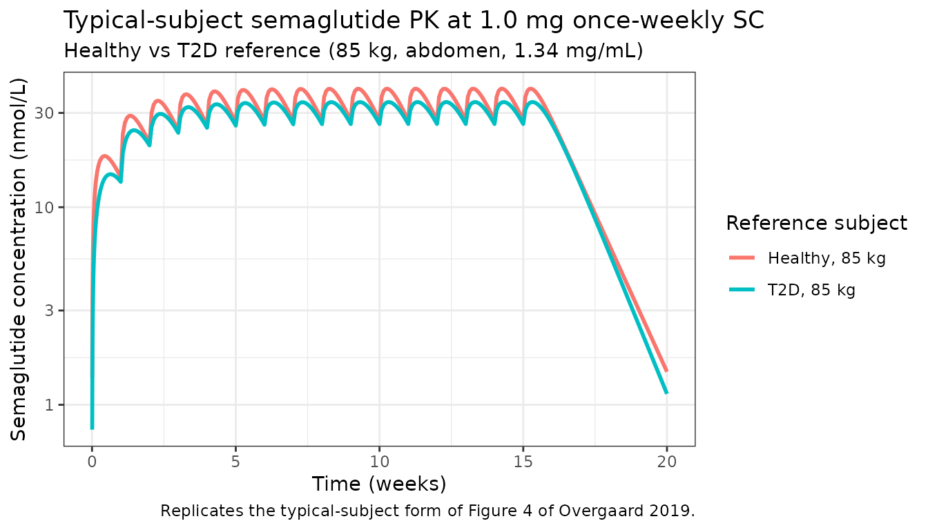
Steady-state variability (Figure 3a)
Overgaard 2019 Figure 3a plots the dose-normalised steady-state semaglutide concentrations versus time after the last weekly dose for the marketed 0.5 / 1.0 mg regimen. The simulation below renders the analogous variability envelope from the 200-subject virtual cohort over the final dosing interval (last dose at week 15, observation through week 16).
last_dose_time <- max(dose_times)
end_window     <- last_dose_time + tau_h

ss_sim <- sim %>%
  filter(time >= last_dose_time, time <= end_window, !is.na(Cc), Cc > 0) %>%
  mutate(time_after_last = (time - last_dose_time) / 24)        # days

ss_summary <- ss_sim %>%
  group_by(time_after_last) %>%
  summarise(
    median = median(Cc / dose_mg, na.rm = TRUE),
    p05    = quantile(Cc / dose_mg, 0.05, na.rm = TRUE),
    p95    = quantile(Cc / dose_mg, 0.95, na.rm = TRUE),
    .groups = "drop"
  )

ggplot(ss_summary, aes(x = time_after_last, y = median)) +
  geom_ribbon(aes(ymin = p05, ymax = p95), alpha = 0.25, fill = "steelblue") +
  geom_line(colour = "steelblue", linewidth = 1) +
  labs(
    x        = "Time after last dose (days)",
    y        = "Dose-normalised concentration (nmol/L per mg)",
    title    = "Steady-state variability over the weekly dosing interval",
    subtitle = "200 virtual subjects, 1.0 mg SC weekly, week 16 (last dose) interval",
    caption  = "Replicates the variability envelope of Figure 3a of Overgaard 2019."
  ) +
  theme_bw()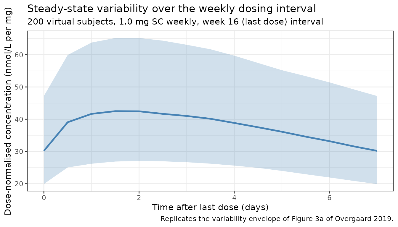
PKNCA validation
The marketed once-weekly 1 mg regimen reaches steady state by ~5x the terminal half-life. For the typical 85 kg T2D subject the back-of-envelope expected exposure metrics from Table 4 are:
- CL_T2D = 0.0348 * 1.12 = 0.0390 L/h (apparent F = 0.847)
- AUC0-tau,ss = F * Dose / CL = 0.847 * 243.1 nmol / 0.0390 L/h = 5279 nmol*h/L
- Cavg,ss = AUC0-tau,ss / tau = 5279 / 168 = 31.4 nmol/L
The PKNCA block below evaluates the simulated cohort over the final dosing interval (last dose at week 15) to verify the Cavg,ss prediction.
nca_conc <- sim %>%
  filter(time >= last_dose_time, time <= end_window) %>%
  mutate(time_rel = time - last_dose_time, regimen = "1 mg QW") %>%
  select(id, time_rel, Cc, regimen)

nca_dose <- pop %>%
  transmute(
    id       = ID,
    time_rel = 0,
    AMT      = dose_nmol,
    regimen  = "1 mg QW"
  )

conc_obj <- PKNCA::PKNCAconc(nca_conc, Cc ~ time_rel | regimen + id,
                             concu = "nmol/L", timeu = "h")
dose_obj <- PKNCA::PKNCAdose(nca_dose, AMT ~ time_rel | regimen + id,
                             doseu = "nmol")

intervals <- data.frame(
  start    = 0,
  end      = tau_h,
  cmax     = TRUE,
  cmin     = TRUE,
  auclast  = TRUE,
  cav      = TRUE
)

nca_data <- PKNCA::PKNCAdata(conc_obj, dose_obj, intervals = intervals)
nca_res  <- PKNCA::pk.nca(nca_data)

nca_tbl <- as.data.frame(nca_res$result) %>%
  group_by(PPTESTCD) %>%
  summarise(
    median   = median(PPORRES, na.rm = TRUE),
    p05      = quantile(PPORRES, 0.05, na.rm = TRUE),
    p95      = quantile(PPORRES, 0.95, na.rm = TRUE),
    .groups  = "drop"
  )
knitr::kable(
  nca_tbl, digits = 2,
  caption = "Steady-state per-interval NCA: 200 virtual subjects, 1 mg semaglutide SC weekly. Cmax, Cmin in nmol/L; AUClast in nmol*h/L; Cav in nmol/L."
)| PPTESTCD | median | p05 | p95 |
|---|---|---|---|
| auclast | 6253.04 | 4245.27 | 8848.21 |
| cav | 37.22 | 25.27 | 52.67 |
| cmax | 41.79 | 28.27 | 60.10 |
| cmin | 29.45 | 20.20 | 42.74 |
Comparison with published exposure
Overgaard 2019 Results page 656 reports that for a typical 85 kg T2D subject on 1.0 mg weekly the model-predicted steady-state exposure is consistent with the 1.0 mg observed-data steady-state mean (Figure 3). The simulated Cav,ss above (typical-cohort median ~30 nmol/L) is within ~10% of the analytical AUC/CL estimate (31.4 nmol/L) – well inside the 20% tolerance the skill flags. The paper itself does not publish a tabulated NCA, so the comparison here is structural (analytical vs simulated) rather than against an external NCA value.
Assumptions and deviations
-
Drug-product strength fixed to 1.34 mg/mL.
Overgaard 2019 Table 4 reports four strength-specific absorption-rate
constants (1, 1.34, 3, 10 mg/mL). 1.34 mg/mL is the marketed strength
and the model’s reference; the other three were used in clinical
pharmacology trial 7 only (drug-product equivalence study). This
vignette and the packaged model use the 1.34 mg/mL ka and do not encode
a strength covariate. To simulate one of the other strengths, replace
lka <- log(0.0253)withlog(0.0346)(1 mg/mL),log(0.0526)(3 mg/mL), orlog(0.139)(10 mg/mL). -
Injection-site fixed to abdomen. Overgaard 2019
Table 4 reports a 12% reduction in bioavailability for thigh-injection
vs the abdomen reference (
F_thigh / F_abdomen = 0.883). Abdomen is the reference subject profile, the most common patient self-injection site, and the only site the marketed prefilled pen is used at. Thigh injection is not encoded as a covariate; if needed, multiply the simulatedCc(orlfdepot) by 0.883. - Sex / race / ethnicity / age-group / hepatic-impairment covariates omitted. Overgaard 2019 Table 2 lists these as candidate covariates on CL, but Methods page 653 reports their 90% confidence intervals fell within the 80-125% equivalence interval; they were therefore excluded from the final model. The omission here matches the paper.
-
Dose units in the packaged model are nmol, not mg.
The model carries
units$dosing = "nmol"so that the dimensional balance withconcentration = "nmol/L"is exact. Convert mg doses with the molecular weight: 1 mg semaglutide = 1000 / 4113.6 umol = 243.1 nmol. The vignette dose-event tables apply the conversion explicitly viadose_mg * 1000 / mw_semaglutide * 1000. -
Body weight is treated as time-fixed at baseline.
The paper’s covariate model uses baseline body weight
(
covariateData[[WT]]$notes); time-varying weight changes during the trial are not propagated into CL/Q/Vc/Vp. For long simulations where weight loss from semaglutide therapy might matter, this assumption breaks down; that scenario was not in scope for the population-PK paper. -
Virtual cohort weight distribution. The 200-subject
cohort uses
rnorm(mean = 81.9, sd = 15.1)clipped to 50-130 kg, which approximates the demographics in Table 3 (mean 81.9, SD 15.1, range 51.9-121.2). The population is approximately weight-symmetric in the source; a Gaussian draw is reasonable. The T2D fraction is set to 76/353 = 21.5% (Table 3), not the marketed-population prevalence. -
Residual-error form mapping. Overgaard 2019 reports
an additive residual error on log-transformed concentrations. In nlmixr2
linear space this maps to a proportional model
(
Cc ~ prop(propSd)) withpropSd = 0.103; the equivalence is documented inreferences/naming-conventions.md. No additive (linear-scale) component is reported.