Liposomal irinotecan and SN-38 PK with exposure-safety (Brendel 2021)
Source:vignettes/articles/Brendel_2021_irinotecan_liposomal.Rmd
Brendel_2021_irinotecan_liposomal.RmdSource and models
Brendel K, Bekaii-Saab T, Boland PM, et al. Population pharmacokinetics of liposomal irinotecan in patients with cancer and exposure-safety analyses in patients with metastatic pancreatic cancer. CPT Pharmacometrics Syst Pharmacol. 2021;10:1550-1563. doi:10.1002/psp4.12725
The paper contributes five models, all documented in this article:
| Model | What it is |
|---|---|
Brendel_2021_irinotecan_liposomal |
Joint popPK model of total irinotecan and SN-38 (Table 2, final NONMEM code in the Supplementary Material) |
Brendel_2021_irinotecan_liposomal_diarrhea_irinotecan |
Logistic model, grade >= 3 diarrhea vs log10 total-irinotecan Cavg,ss (Figure 4a) |
Brendel_2021_irinotecan_liposomal_diarrhea_sn38 |
Logistic model, grade >= 3 diarrhea vs log10 SN-38 Cavg,ss (Figure 4b) |
Brendel_2021_irinotecan_liposomal_neutropenia_irinotecan |
Logistic model, grade >= 3 neutropenia AEs vs log10 total-irinotecan Cavg,ss (Figure 5a) |
Brendel_2021_irinotecan_liposomal_neutropenia_sn38 |
Logistic model, grade >= 3 neutropenia AEs vs log10 SN-38 Cavg,ss (Figure 5b) |
An earlier analysis of 353 of the same patients,
Adiwijaya_2017_irinotecan_liposomal, fits the two analytes
sequentially and with a different structure; Brendel 2021 replaced it
with this joint parent-metabolite model.
mod_pk <- readModelDb("Brendel_2021_irinotecan_liposomal")
er_names <- c(
  diarrhea_irinotecan = "Brendel_2021_irinotecan_liposomal_diarrhea_irinotecan",
  diarrhea_sn38 = "Brendel_2021_irinotecan_liposomal_diarrhea_sn38",
  neutropenia_irinotecan = "Brendel_2021_irinotecan_liposomal_neutropenia_irinotecan",
  neutropenia_sn38 = "Brendel_2021_irinotecan_liposomal_neutropenia_sn38"
)
mod_er <- lapply(er_names, readModelDb)
ui_pk <- rxode2::rxode(mod_pk)
#> ℹ parameter labels from comments will be replaced by 'label()'
Population
The popPK model was fit to 440 patients from seven studies (Table 1): the phase III NAPOLI-1 trial (N = 260, second-line metastatic pancreatic ductal adenocarcinoma, mPDAC), the phase I/II first-line mPDAC study NCT02551991 (N = 56, with 5-FU/LV and oxaliplatin), and five phase I/II studies in various solid tumours or metastatic colorectal cancer (N = 124). Doses ranged from 35 to 156 mg/m^2 irinotecan free base every 2 or 3 weeks, given as a 90-minute infusion. Supplementary Table S1: median age 62 years (28-87), median BSA 1.71 m^2 (1.29-2.48), 48.6% female, 35.2% Asian, median bilirubin 0.41 mg/dL, median creatinine clearance 85 mL/min, 12.7% on oxaliplatin, 6.1% UGT1A1*28 7/7 homozygous, and 18.6% treated with product from the previous manufacturing site.
The exposure-safety analyses used the 316 mPDAC patients of NAPOLI-1 and NCT02551991, one record each (the first grade >= 3 event, if any).
str(ui_pk$population)
#> List of 14
#>  $ species         : chr "human"
#>  $ n_subjects      : int 440
#>  $ n_studies       : int 7
#>  $ age_median      : chr "62 years"
#>  $ age_range       : chr "28-87 years"
#>  $ sex_female_pct  : num 48.6
#>  $ race_ethnicity  : Named num [1:2] 35.2 64.8
#>   ..- attr(*, "names")= chr [1:2] "Asian" "non-Asian"
#>  $ disease_state   : chr "Advanced solid tumours: metastatic pancreatic ductal adenocarcinoma (NAPOLI-1, N = 260; NCT02551991, N = 56), m"| __truncated__
#>  $ dose_range      : chr "35-156 mg/m^2 irinotecan free base (40-180 mg/m^2 irinotecan hydrochloride trihydrate) as a 90-minute intraveno"| __truncated__
#>  $ bsa_median      : chr "1.71 m^2 (range 1.29-2.48)"
#>  $ hepatic_function: chr "Bilirubin median 0.41 mg/dL (range 0.12-2.11); ALT median 24 IU/L (4-202); albumin median 4 g/dL (2.1-5.1)"
#>  $ renal_function  : chr "Creatinine clearance median 85 mL/min (range 27-177)"
#>  $ co_medication   : chr "5-FU/LV 42.7%; oxaliplatin (with 5-FU/LV) 12.7%"
#>  $ notes           : chr "Baseline covariates from Supplementary Table S1; study designs from Table 1. 1887 total-irinotecan and 1827 SN-"| __truncated__
Source trace
Every value in the popPK model is in Table 2, which is identical to Supplementary Table S3; the equations are from the final NONMEM control stream printed in the Supplementary Material.
| Quantity | Value | Source |
|---|---|---|
| Structure: 2-cmt irinotecan, 1-cmt SN-38, direct + one-transit formation | – | Figure 1; control stream $MODEL, $PK
|
FM1 = FR1/(1+FR1+FR2),
FM2 = FR2/(1+FR1+FR2)
|
– | control stream $PK
|
| SN-38 volume = irinotecan central volume | – | Methods (Base model); control stream VCM = VCP
|
Scale: irinotecan A1/V, SN-38
A2/(V/1000)
|
– | control stream S1, S2
|
lcl irinotecan CL |
17.9 L/week | Table 2 |
lvc irinotecan central volume |
4.09 L | Table 2 |
lq intercompartmental clearance |
1.35 L/week | Table 2 |
lvp peripheral volume |
0.421 L | Table 2 |
lfr1 direct pathway ratio FR1 |
0.152 | Table 2, ‘Fraction of direct …’ |
lfr2 delayed pathway ratio FR2 |
0.629 | Table 2, ‘Fraction of delayed …’ |
lktr transformation rate after delay |
2 1/week | Table 2 |
lcl_sn38 SN-38 clearance |
19,800 L/week | Table 2 |
| CL: Asian / previous site / female / oxaliplatin | x 1.204 / 1.515 / 0.799 / 1.339 | Table 2 |
| V: BSA exponent / previous site / female | (BSA/1.71)^0.573 / x 0.872 / 0.886 | Table 2 |
| FR2: previous site | x 1.376 | Table 2 |
| CL SN-38: bilirubin / CrCL / female / oxaliplatin | (BIL/0.41)^-0.266 / (CrCL/85.04)^0.25 / x 0.802 / 0.656 | Table 2 |
| IIV variances CL, V, FR1, FR2, KTR, CL SN-38 | 0.545, 0.066, 0.928, 0.188, 0.135, 0.126 | Table 2 |
| Covariances CL-V, CL-FR1, V-FR1 | 0.117, -0.558, -0.103 | Table 2 |
| Proportional error irinotecan / SN-38 | 0.243 / 0.291 | Table 2 |
| Irinotecan free-base molecular weight | 586.678 g/mol | Methods (Study data) |
| SN-38 molecular weight | 392.41 g/mol | not printed; computed from C22H20N2O5 |
| Diarrhea odds ratios (irinotecan / SN-38), per log10 Cavg,ss | 8.70 / 7.30 | Results, Diarrhea; Figure 4 |
| Neutropenia odds ratios (irinotecan / SN-38), per log10 Cavg,ss | 0.33 / 3.14 | Results, Neutropenia AEs; Figure 5 |
| Four logistic intercepts | -2.663, -1.575, -0.621, -1.165 | digitised from Figures 4a, 4b, 5a, 5b |
Two checks on the transcription: every printed %CV equals
sqrt(exp(omega^2) - 1) for its variance, and every printed
correlation equals the covariance divided by the root product of its two
variances.
om <- c(cl = 0.545, vc = 0.066, fr1 = 0.928, fr2 = 0.188, ktr = 0.135, cl_sn38 = 0.126)
cv_printed <- c(85.2, 26.1, 124, 45.4, 38, 36.6)
cv_calc <- 100 * sqrt(exp(om) - 1)
rbind(printed = cv_printed, computed = round(cv_calc, 1))
#>            cl   vc   fr1  fr2 ktr cl_sn38
#> printed  85.2 26.1 124.0 45.4  38    36.6
#> computed 85.1 26.1 123.7 45.5  38    36.6
stopifnot(max(abs(cv_calc - cv_printed) / cv_printed) < 0.005)

cor_calc <- c(
  cl_fr1 = -0.558 / sqrt(0.545 * 0.928),
  cl_vc = 0.117 / sqrt(0.545 * 0.066),
  vc_fr1 = -0.103 / sqrt(0.066 * 0.928)
)
rbind(printed = c(-0.785, 0.617, -0.416), computed = round(cor_calc, 3))
#>          cl_fr1 cl_vc vc_fr1
#> printed  -0.785 0.617 -0.416
#> computed -0.785 0.617 -0.416
stopifnot(max(abs(cor_calc - c(-0.785, 0.617, -0.416))) < 0.002)

# The typical-value fractions of irinotecan elimination forming SN-38 match
# the Results ('one direct ... (9%) and one delayed via a transit
# compartment (35%)').
fm <- c(direct = 0.152, delayed = 0.629) / (1 + 0.152 + 0.629)
round(100 * fm, 1)
#>  direct delayed
#>     8.5    35.3
stopifnot(abs(100 * fm[["direct"]] - 9) < 0.5, abs(100 * fm[["delayed"]] - 35) < 0.5)
Concentration units
The Results state that the joint model was developed with both
analytes in molar units, and the control stream’s SN-38 scale
S2 = VCP/1000 turns micromoles and litres into nmol/L. The
paper’s figures, however, are in ug/mL (irinotecan) and ng/mL (SN-38).
Because irinotecan is converted to SN-38 one molecule for one molecule,
only the SN-38 prediction depends on which units the model was fitted
in: read in mass units, it would be 586.678 / 392.41 = 1.50-fold higher
than read in molar units. Every parameter value is the same under both
readings.
The model file follows the molar reading. It takes doses in mg of free base and reports irinotecan in ug/mL, and it multiplies the SN-38 formation flux by the molecular-weight ratio before reporting SN-38 in ng/mL. Besides the Results statement, the paper’s own model-derived exposures support this choice. The median post hoc SN-38 Cavg,ss in Figures 4b and 5b sits at log10 = -0.025; the molar reading reproduces it, and the mass reading lands 0.175 log10 units (50%) higher (see the steady-state section below). Total irinotecan, where the two readings agree, reproduces the Figure 4a median, which shows that the virtual cohort and dosing are right. The Figure 3 VPC does not discriminate between the readings: its SN-38 to irinotecan ratios fall between the two, closer to one in some bins and to the other in others.
Virtual cohort
The cohort mirrors the exposure-safety population: NAPOLI-1 liposomal irinotecan 100 mg/m^2 Q3W alone, 70 mg/m^2 Q2W with 5-FU/LV, and NCT02551991 50 mg/m^2 Q2W with 5-FU/LV and oxaliplatin (NALIRIFOX). Arm sizes keep the paper’s roughly 260:56 split between NAPOLI-1 and NCT02551991, which matters for the pooled comparison with Figure 4. All patients receive product from the current manufacturing site. Covariates are sampled to match Supplementary Table S1.
set.seed(20211215)
rxode2::rxSetSeed(20211215)

arms <- tibble::tribble(
  ~treatment,                      ~n,  ~dose_mgm2, ~tau, ~oxa,
  "NAPOLI-1 100 mg/m2 Q3W",        140, 100,         3,    0L,
  "NAPOLI-1 70 mg/m2 Q2W + 5-FU",  120,  70,         2,    0L,
  "NALIRIFOX 50 mg/m2 Q2W",         56,  50,         2,    1L
)
stopifnot(all(arms$n <= 200))

rtrunc <- function(n, mean, sd, lo, hi) pmin(pmax(rnorm(n, mean, sd), lo), hi)

cohort <- arms |>
  tidyr::uncount(n) |>
  mutate(
    id = dplyr::row_number(),
    BSA = rtrunc(dplyr::n(), 1.73, 0.22, 1.29, 2.48),
    SEXF = rbinom(dplyr::n(), 1, 0.486),
    RACE_ASIAN = rbinom(dplyr::n(), 1, 0.352),
    TBILI = 17.1 * exp(rtrunc(dplyr::n(), log(0.41), 0.4, log(0.12), log(2.11))),
    CRCL = rtrunc(dplyr::n(), 88, 30, 27, 177),
    CONMED_OXALIPLATIN = oxa,
    FORM_NALIRI_PREVSITE = 0L,
    amt = dose_mgm2 * BSA
  )
cohort |>
  summarise(
    n = dplyr::n(), `median BSA` = median(BSA), `% female` = 100 * mean(SEXF),
    `% Asian` = 100 * mean(RACE_ASIAN), `median bilirubin (mg/dL)` = median(TBILI / 17.1),
    `median CrCL (mL/min)` = median(CRCL), `% oxaliplatin` = 100 * mean(CONMED_OXALIPLATIN)
  ) |>
knitr::kable(digits = 2)| n | median BSA | % female | % Asian | median bilirubin (mg/dL) | median CrCL (mL/min) | % oxaliplatin |
|---|---|---|---|---|---|---|
| 316 | 1.72 | 51.27 | 35.76 | 0.43 | 88.44 | 17.72 |
Simulation
Four cycles are simulated. Cycle 1 carries the profile for Figure 3;
cycle 4 is at steady state and carries the Cavg,ss for Figures 4 and 5.
Time is in weeks. The model has two endpoints, so observation rows carry
dvid = 1, which returns both Cc and
Cc_sn38 on every row.
inf_dur <- 1.5 / 168 # 90-minute infusion, in weeks
grid_h <- c(0, 0.5, 1, 1.5, 2, 2.5, 3.5, 4.5, 6, 8, 12, 18, 24, 36, 48, 72, 96, 120, 168, 216, 264, 336, 408, 504)

make_events <- function(cohort) {
  doses <- cohort |>
    tidyr::crossing(cycle = 0:3) |>
    transmute(id, time = cycle * tau, amt, rate = amt / inf_dur, evid = 1L, cmt = "central", dvid = NA_integer_)
  obs <- cohort |>
    tidyr::crossing(cycle = c(0L, 3L), h = grid_h) |>
    filter(h <= tau * 168) |>
    transmute(id, time = cycle * tau + h / 168, amt = 0, rate = 0, evid = 0L, cmt = "central", dvid = 1L) |>
    distinct()
  covs <- cohort |> select(id, treatment, tau, BSA, SEXF, RACE_ASIAN, TBILI, CRCL, CONMED_OXALIPLATIN, FORM_NALIRI_PREVSITE)
  bind_rows(doses, obs) |>
    arrange(id, time, desc(evid)) |>
    left_join(covs, by = "id")
}
ev <- make_events(cohort)

sim <- as.data.frame(rxode2::rxSolve(
  mod_pk,
  events = ev,
  returnType = "data.frame",
  keep = c("treatment", "tau"),
  maxsteps = 1e6
))
#> ℹ parameter labels from comments will be replaced by 'label()'
stopifnot(!anyNA(sim$Cc), !anyNA(sim$Cc_sn38))
# LSODA undershoots zero by solver noise in the far tail; assert it is noise.
stopifnot(all(sim$Cc >= -1e-6 * max(sim$Cc)), all(sim$Cc_sn38 >= -1e-6 * max(sim$Cc_sn38)))
sim <- sim |> mutate(Cc = pmax(Cc, 0), Cc_sn38 = pmax(Cc_sn38, 0))
Replicate Figure 3 (first-cycle profiles)
Figure 3 is a prediction-corrected VPC over the first week after a dose, pooled over all seven studies and dose levels. The points below are the simulated medians of Figure 3, digitised by the maintainers at each bin’s mid-time; they are a guide, not a target, because the cohort here is the mPDAC subset only and the figure is prediction-corrected.
fig3 <- tibble::tribble(
  ~analyte,      ~time,  ~median,
  "irinotecan",  0.020,  29,
  "irinotecan",  0.095,  27,
  "irinotecan",  0.208,  12,
  "irinotecan",  0.333,  7.0,
  "irinotecan",  0.508,  4.7,
  "irinotecan",  0.804,  1.5,
  "SN-38",       0.020,  2.3,
  "SN-38",       0.095,  3.6,
  "SN-38",       0.208,  4.2,
  "SN-38",       0.333,  2.6,
  "SN-38",       0.508,  2.6,
  "SN-38",       0.804,  1.05
)

c1 <- sim |>
  filter(time > 0, time <= 1) |>
  select(id, time, `irinotecan` = Cc, `SN-38` = Cc_sn38) |>
  pivot_longer(c(`irinotecan`, `SN-38`), names_to = "analyte", values_to = "conc") |>
  group_by(analyte, time) |>
  summarise(
    p05 = quantile(conc, 0.05), p50 = median(conc), p95 = quantile(conc, 0.95),
    .groups = "drop"
  )

ggplot(c1, aes(time, p50)) +
  geom_ribbon(aes(ymin = p05, ymax = p95), alpha = 0.25) +
  geom_line() +
  geom_point(data = fig3, aes(time, median), colour = "red", size = 2) +
  scale_y_log10() +
  facet_wrap(~analyte, ncol = 1, scales = "free_y") +
  labs(
    x = "Time after dose (weeks)",
    y = "Concentration (irinotecan ug/mL; SN-38 ng/mL)",
    caption = "Replicates Figure 3 of Brendel 2021. Line and band: simulated median and 5th-95th percentiles.\nRed points: simulated medians of Figure 3, digitised."
  )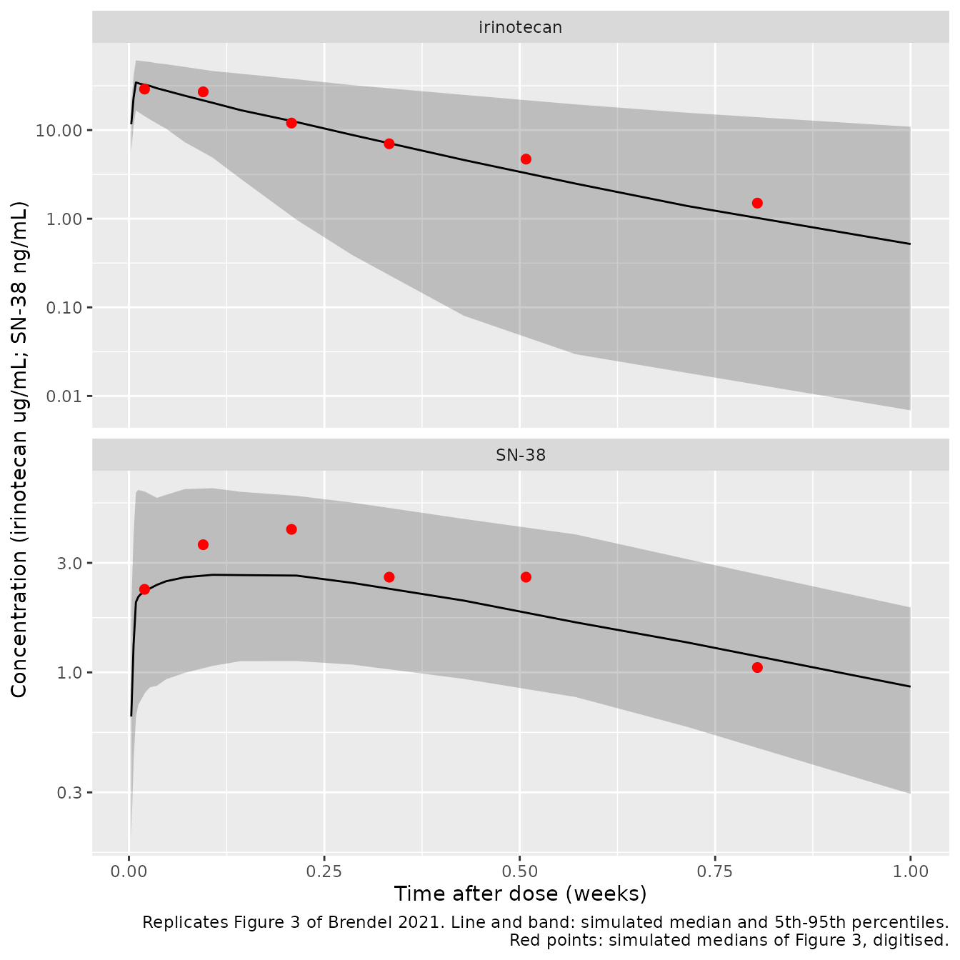
The SN-38 to irinotecan ratio at each bin cancels the dose and most covariates, so it is the part of Figure 3 that bears on the unit reading. It is not decisive: the published ratios lie between the molar and mass readings, nearer the molar one in some bins and nearer the mass one in others. The comparison uses the simulated median at the grid time nearest each bin centre, and the figure is prediction-corrected and pools all seven studies, so bin-level agreement is only approximate.
ratio_tab <- fig3 |>
  pivot_wider(names_from = analyte, values_from = median) |>
  mutate(paper = `SN-38` / irinotecan) |>
  select(time, paper) |>
  left_join(
    c1 |>
      select(analyte, time, p50) |>
      pivot_wider(names_from = analyte, values_from = p50) |>
      mutate(time_bin = time) |>
      select(time_bin, irinotecan, `SN-38`),
    by = join_by(closest(time >= time_bin))
  ) |>
  mutate(
    `molar reading` = `SN-38` / irinotecan,
    `mass reading` = `molar reading` * 586.678 / 392.41
  ) |>
  select(`Time (weeks)` = time, `Figure 3 ratio` = paper, `molar reading`, `mass reading`)
knitr::kable(ratio_tab, digits = 3)| Time (weeks) | Figure 3 ratio | molar reading | mass reading |
|---|---|---|---|
| 0.020 | 0.079 | 0.066 | 0.099 |
| 0.095 | 0.133 | 0.106 | 0.159 |
| 0.208 | 0.350 | 0.158 | 0.236 |
| 0.333 | 0.371 | 0.279 | 0.417 |
| 0.508 | 0.553 | 0.447 | 0.668 |
| 0.804 | 0.700 | 0.970 | 1.451 |
Steady-state exposure and PKNCA
PKNCA computes each patient’s average concentration over the last
dosing interval (cycle 4). With linear kinetics, Cavg,ss has closed
forms, Dose / (CL * tau) for irinotecan and
1000 * MW ratio * (FM1 + FM2) * Dose / (CL_SN38 * tau) for
SN-38. PKNCA must reproduce them.
ss <- sim |>
  filter(time >= 3 * tau - 1e-9) |>
  mutate(treatment = factor(treatment, levels = arms$treatment))
# Time-zero row of each steady-state interval is present by construction.
stopifnot(all(tapply(abs(ss$time - 3 * ss$tau) < 1e-9, ss$id, any)))

doses_ss <- ev |>
  filter(evid == 1, abs(time - 3 * tau) < 1e-9) |>
  mutate(treatment = factor(treatment, levels = arms$treatment)) |>
  select(id, time, amt, treatment)

intervals <- arms |>
  transmute(
    treatment = factor(treatment, levels = arms$treatment),
    start = 3 * tau, end = 4 * tau, cav = TRUE, cmax = TRUE, auclast = TRUE
  )

run_nca <- function(conc_col) {
  conc <- ss |>
    select(id, time, treatment, conc = all_of(conc_col)) |>
    filter(!is.na(conc))
  o_conc <- PKNCA::PKNCAconc(conc, conc ~ time | treatment + id)
  o_dose <- PKNCA::PKNCAdose(doses_ss, amt ~ time | treatment + id)
  res <- PKNCA::pk.nca(PKNCA::PKNCAdata(o_conc, o_dose, intervals = as.data.frame(intervals)))
  as.data.frame(res$result)
}
nca_iri <- run_nca("Cc")
nca_sn38 <- run_nca("Cc_sn38")

indiv <- sim |>
  group_by(id) |>
  slice(1) |>
  ungroup() |>
  select(id, treatment, tau, cl, cl_sn38, fm1, fm2) |>
  left_join(cohort |> select(id, amt), by = "id") |>
  mutate(
    cav_iri_cf = amt / (cl * tau),
    cav_sn38_cf = 1000 * (392.41 / 586.678) * (fm1 + fm2) * amt / (cl_sn38 * tau)
  ) |>
  left_join(nca_iri |> filter(PPTESTCD == "cav") |> select(id, cav_iri = PPORRES), by = "id") |>
  left_join(nca_sn38 |> filter(PPTESTCD == "cav") |> select(id, cav_sn38 = PPORRES), by = "id")
stopifnot(nrow(indiv) == nrow(cohort), !anyNA(indiv$cav_iri), !anyNA(indiv$cav_sn38))

err <- indiv |>
  summarise(
    irinotecan_median = median(100 * (cav_iri / cav_iri_cf - 1)),
    irinotecan_p90 = quantile(abs(100 * (cav_iri / cav_iri_cf - 1)), 0.9),
    sn38_median = median(100 * (cav_sn38 / cav_sn38_cf - 1)),
    sn38_p90 = quantile(abs(100 * (cav_sn38 / cav_sn38_cf - 1)), 0.9)
  )
knitr::kable(err, digits = 2, caption = "PKNCA Cavg,ss versus the closed form (% difference)")| irinotecan_median | irinotecan_p90 | sn38_median | sn38_p90 |
|---|---|---|---|
| 0.13 | 0.18 | -0.21 | 0.43 |
# The two sides use the same drawn parameters, so the difference is
# trapezoid error plus the small residual accumulation of slow-clearing
# patients after three doses. A mis-coded formation fraction, molecular-weight
# ratio or clearance moves these by tens of percent.
stopifnot(abs(err$irinotecan_median) < 2, err$irinotecan_p90 < 6)
stopifnot(abs(err$sn38_median) < 2, err$sn38_p90 < 6)
Comparison with the published exposure distribution
The paper gives no NCA table; the only published exposure values are the Cavg,ss quartiles of the 316 exposure-safety patients, drawn as vertical lines in Figures 4 and 5. Their median is log10 0.50 (3.16 ug/mL) for total irinotecan and log10 -0.025 (0.944 ng/mL) for SN-38.
sim_cav <- bind_rows(
  nca_iri |> filter(PPTESTCD == "cav") |> mutate(analyte = "Total irinotecan (ug/mL)"),
  nca_sn38 |> filter(PPTESTCD == "cav") |> mutate(analyte = "SN-38 (ng/mL)")
) |>
  select(analyte, PPTESTCD, PPORRES)
ref_cav <- data.frame(
  analyte = c("Total irinotecan (ug/mL)", "SN-38 (ng/mL)"),
  cav = 10^c(0.50, -0.025)
)
knitr::kable(ncaComparisonTable(sim_cav, ref_cav, by = "analyte"), digits = 3)| NCA parameter | analyte | Reference | Simulated | % diff |
|---|---|---|---|---|
| Cavg | Total irinotecan (ug/mL) | 3.16 | 3.03 | -4.2% |
| Cavg | SN-38 (ng/mL) | 0.944 | 1.07 | +13.1% |
q_sim <- rbind(
  irinotecan = quantile(log10(indiv$cav_iri), c(0.25, 0.5, 0.75)),
  sn38_molar = quantile(log10(indiv$cav_sn38), c(0.25, 0.5, 0.75)),
  sn38_mass = quantile(log10(indiv$cav_sn38 * 586.678 / 392.41), c(0.25, 0.5, 0.75))
)
q_paper <- rbind(irinotecan = c(0.33, 0.50, 0.68), sn38 = c(-0.12, -0.025, 0.095))
knitr::kable(
  data.frame(
    Quantity = c("Total irinotecan", "SN-38, molar reading (model)", "SN-38, mass reading"),
    `Simulated Q1` = q_sim[, 1], `Simulated median` = q_sim[, 2], `Simulated Q3` = q_sim[, 3],
    `Figure 4 Q1` = q_paper[c(1, 2, 2), 1], `Figure 4 median` = q_paper[c(1, 2, 2), 2],
    `Figure 4 Q3` = q_paper[c(1, 2, 2), 3],
    check.names = FALSE
  ),
  digits = 3, row.names = FALSE,
  caption = "log10 Cavg,ss quartiles: simulated cohort against Figures 4 and 5"
)| Quantity | Simulated Q1 | Simulated median | Simulated Q3 | Figure 4 Q1 | Figure 4 median | Figure 4 Q3 |
|---|---|---|---|---|---|---|
| Total irinotecan | 0.243 | 0.481 | 0.794 | 0.33 | 0.500 | 0.680 |
| SN-38, molar reading (model) | -0.099 | 0.029 | 0.146 | -0.12 | -0.025 | 0.095 |
| SN-38, mass reading | 0.076 | 0.203 | 0.320 | -0.12 | -0.025 | 0.095 |
# Median on the log10 scale: 0.1 is 26% on the concentration scale. The
# molar/mass readings differ by 0.175, so the gate discriminates them.
stopifnot(
  abs(q_sim["irinotecan", 2] - 0.50) < 0.1,
  abs(q_sim["sn38_molar", 2] - (-0.025)) < 0.1
)
The simulated interquartile ranges are wider than the published ones. That is expected: the published quartiles come from post hoc (empirical Bayes) estimates, which shrink towards the typical value, while the simulation draws the full between-patient variability.
Replicate Figures 4 and 5 (exposure-safety)
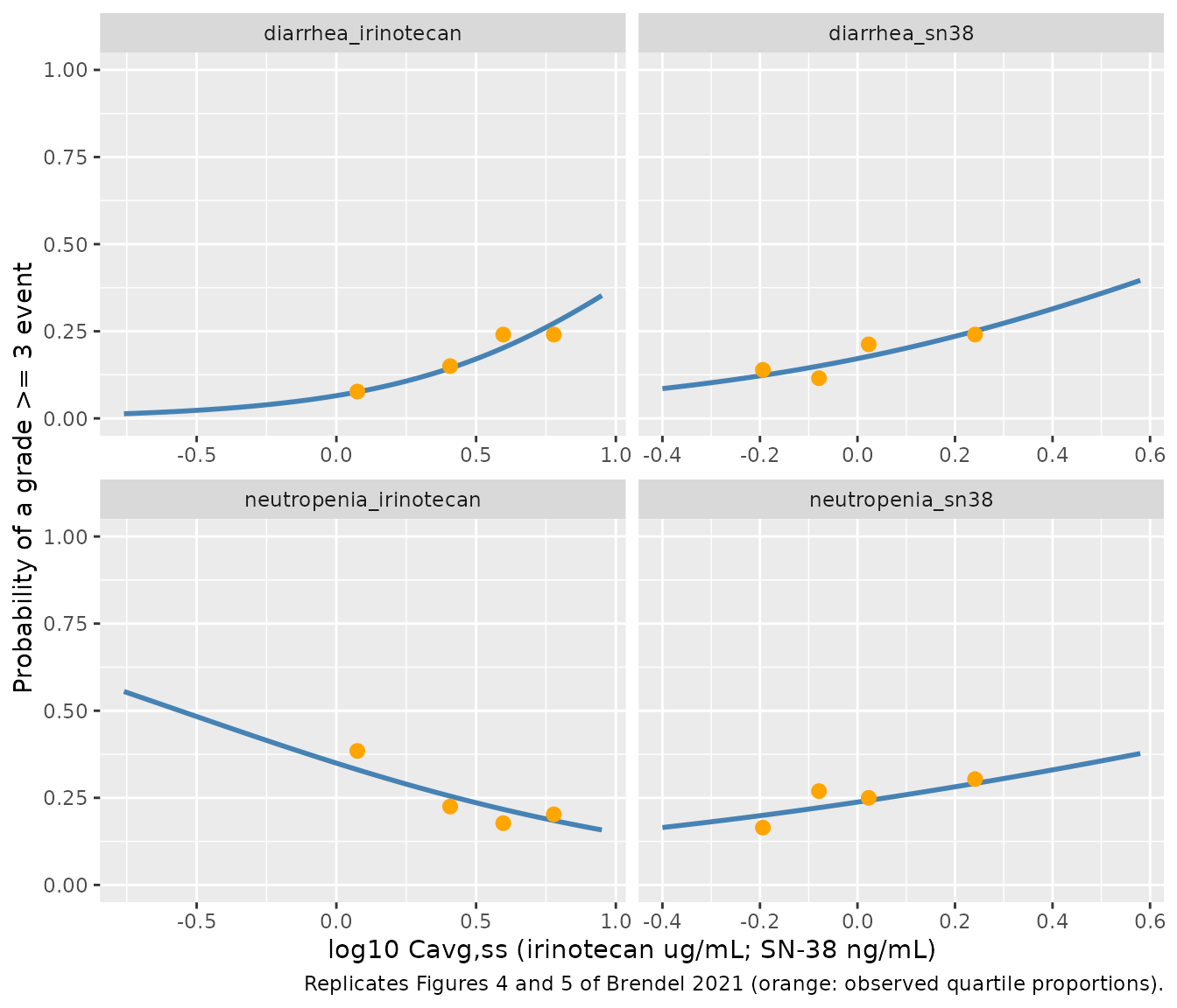
The four logistic models are univariable in log10 Cavg,ss. The figures plot the fitted curve over each analyte’s observed range, with the observed proportion of patients with an event in each exposure quartile. Those quartile points and their counts are printed in the figures and are overlaid here.
# The landmark models have no random effects, so rxode2 notes that a
# multi-subject solve has no omega; that note is expected and muffled.
muffle_no_omega <- function(w) {
  if (grepl("without 'omega'", conditionMessage(w), fixed = TRUE)) invokeRestart("muffleWarning")
}
solve_prob <- function(model, cav) {
  out <- withCallingHandlers(
    rxode2::rxSolve(
      model,
      events = data.frame(id = seq_along(cav), time = 0, amt = 0, evid = 0L, CAV = cav),
      returnType = "data.frame"
    ),
    warning = muffle_no_omega
  )
  out <- as.data.frame(out)
  pcol <- grep("^prob_", names(out), value = TRUE)
  stopifnot(length(pcol) == 1L, nrow(out) == length(cav))
  out[[pcol]]
}

ranges <- list(irinotecan = c(-0.76, 0.95), sn38 = c(-0.40, 0.58))
curves <- bind_rows(lapply(names(mod_er), function(nm) {
  an <- sub("^[a-z]+_", "", nm)
  x <- seq(ranges[[an]][1], ranges[[an]][2], length.out = 60)
  tibble::tibble(model = nm, log10_cav = x, p = solve_prob(mod_er[[nm]], 10^x))
}))

# Observed quartile points (x at the digitised point position; n and
# events as printed under each figure panel).
quart <- tibble::tribble(
  ~model,                    ~log10_cav, ~events, ~n,
  "diarrhea_irinotecan",      0.075,      6,      78,
  "diarrhea_irinotecan",      0.407,     12,      80,
  "diarrhea_irinotecan",      0.597,     19,      79,
  "diarrhea_irinotecan",      0.778,     19,      79,
  "diarrhea_sn38",           -0.194,     11,      79,
  "diarrhea_sn38",           -0.079,      9,      78,
  "diarrhea_sn38",            0.023,     17,      80,
  "diarrhea_sn38",            0.241,     19,      79,
  "neutropenia_irinotecan",   0.075,     30,      78,
  "neutropenia_irinotecan",   0.407,     18,      80,
  "neutropenia_irinotecan",   0.597,     14,      79,
  "neutropenia_irinotecan",   0.778,     16,      79,
  "neutropenia_sn38",        -0.194,     13,      79,
  "neutropenia_sn38",        -0.079,     21,      78,
  "neutropenia_sn38",         0.023,     20,      80,
  "neutropenia_sn38",         0.241,     24,      79
) |>
  mutate(observed = events / n)

ggplot(curves, aes(log10_cav, p)) +
  geom_line(colour = "steelblue", linewidth = 1) +
  geom_point(data = quart, aes(y = observed), colour = "orange", size = 2.5) +
  facet_wrap(~model, scales = "free_x") +
  coord_cartesian(ylim = c(0, 1)) +
  labs(
    x = "log10 Cavg,ss (irinotecan ug/mL; SN-38 ng/mL)",
    y = "Probability of a grade >= 3 event",
    caption = "Replicates Figures 4 and 5 of Brendel 2021 (orange: observed quartile proportions)."
  )
Intercept check
For a logistic regression fitted by maximum likelihood, the predicted probabilities summed over the analysis set equal the number of events exactly. Approximating each patient’s exposure by the position of their quartile’s point, the digitised intercepts must therefore return close to the printed totals: 56 of 316 diarrhea events (17.7%) and 78 of 316 neutropenia events (24.7%). This check does not use the digitised curves, only the printed counts and the printed odds ratios.
chk <- quart |>
  group_by(model) |>
  group_modify(function(d, key) {
    p <- solve_prob(mod_er[[key$model]], 10^d$log10_cav)
    tibble::tibble(
      events_obs = sum(d$events), events_pred = sum(d$n * p), n = sum(d$n),
      max_bin_diff_pct = max(abs(100 * (p - d$observed)))
    )
  }) |>
  ungroup() |>
  mutate(
    pct_obs = 100 * events_obs / n, pct_pred = 100 * events_pred / n,
    diff_pct_points = pct_pred - pct_obs
  )
knitr::kable(chk, digits = 2)| model | events_obs | events_pred | n | max_bin_diff_pct | pct_obs | pct_pred | diff_pct_points |
|---|---|---|---|---|---|---|---|
| diarrhea_irinotecan | 56 | 54.98 | 316 | 3.81 | 17.72 | 17.40 | -0.32 |
| diarrhea_sn38 | 56 | 55.51 | 316 | 3.49 | 17.72 | 17.57 | -0.15 |
| neutropenia_irinotecan | 78 | 77.96 | 316 | 5.37 | 24.68 | 24.67 | -0.01 |
| neutropenia_sn38 | 78 | 75.50 | 316 | 4.75 | 24.68 | 23.89 | -0.79 |
stopifnot(all(chk$events_obs == c(56, 56, 78, 78)))
# The within-quartile spread of exposure makes the quartile-point
# approximation inexact; a misread intercept moves this by far more
# (0.5 on the logit scale shifts the diarrhea totals by about 7 points).
stopifnot(all(abs(chk$diff_pct_points) < 2))
The reported odds ratios can also be checked against the printed
percentage changes: an odds ratio of 8.70 per log10 unit means a
doubling of total irinotecan Cavg,ss raises the odds of grade >= 3
diarrhea by 8.70^log10(2) = 1.92-fold.
Predicted incidence in the virtual cohort
inc <- indiv |>
  mutate(
    diarrhea_irinotecan = solve_prob(mod_er$diarrhea_irinotecan, cav_iri),
    diarrhea_sn38 = solve_prob(mod_er$diarrhea_sn38, cav_sn38),
    neutropenia_irinotecan = solve_prob(mod_er$neutropenia_irinotecan, cav_iri),
    neutropenia_sn38 = solve_prob(mod_er$neutropenia_sn38, cav_sn38)
  ) |>
  group_by(treatment) |>
  summarise(across(diarrhea_irinotecan:neutropenia_sn38, \(x) 100 * mean(x)), .groups = "drop")
knitr::kable(inc, digits = 1, caption = "Mean predicted probability (%) of a grade >= 3 event by arm")| treatment | diarrhea_irinotecan | diarrhea_sn38 | neutropenia_irinotecan | neutropenia_sn38 |
|---|---|---|---|---|
| NALIRIFOX 50 mg/m2 Q2W | 14.5 | 18.9 | 29.9 | 24.8 |
| NAPOLI-1 100 mg/m2 Q3W | 21.5 | 18.1 | 23.1 | 24.2 |
| NAPOLI-1 70 mg/m2 Q2W + 5-FU | 20.8 | 18.3 | 23.2 | 24.4 |
The paper reports 16.9% (NAPOLI-1) and 21.4% (NCT02551991) grade >= 3 diarrhea, and 20.8% and 42.9% grade >= 3 neutropenia AEs. The univariable exposure models do not carry that difference between studies. The irinotecan neutropenia model does predict more neutropenia on NALIRIFOX, because the lower dose and the oxaliplatin-driven rise in irinotecan clearance lower irinotecan exposure and the fitted relationship is inverse, but it falls well short of the observed 42.9%. The authors call the inverse irinotecan-neutropenia relationship unexpected, and the SN-38 neutropenia relationship is not statistically significant (p = 0.115). These models describe association in the pooled data; they are not a basis for predicting the effect of adding oxaliplatin.
Assumptions and deviations
- Molar model, mass outputs. Doses are mg of irinotecan free base; the SN-38 formation flux is multiplied by 392.41 / 586.678 so that SN-38 is reported in ng/mL. The SN-38 molecular weight is not in the paper; it was computed from the formula C22H20N2O5 with standard atomic weights. See “Concentration units” for why the molar reading was chosen.
-
Covariate coding. Categorical effects are coded
exactly as in the control stream,
(1 + THETA * indicator); the model file stores THETA = printed factor - 1. The control stream codes manufacturing site with the current site asMFG = 1, soFORM_NALIRI_PREVSITE = 1 - MFG.SEX = 1is female. The control stream sets the bilirubin and creatinine-clearance effects to 1 when either value is missing (-99); impute the medians (0.41 mg/dL, 85.04 mL/min) to reproduce that. -
Bilirubin units. The canonical
TBILIcolumn is in umol/L; the model divides by 17.1 to recover the source’s mg/dL before applying(BIL / 0.41)^-0.266. - Creatinine clearance is absolute mL/min, as in the source; the estimating equation is not reported.
-
Correlated residual error not encoded. The control
stream estimates a correlation of 0.323 between the irinotecan and SN-38
residuals by reusing
EPS(1)on SN-38 records. Irinotecan and SN-38 are separate records in the data, so their residual draws are independent and the correlation cannot act; the SN-38 residual variance is0.291^2either way. nlmixr2 has no cross-endpoint residual correlation, so only the two proportional errors are encoded. - Data below the limit of quantification were discarded in the final model (M1), with 23% of irinotecan and 25% of SN-38 samples below the limit. This does not change the model, but explains why Figure 3’s late observed medians sit above the simulated ones.
- Exposure-safety intercepts are digitised. The paper prints only the odds ratios and p values. The intercepts were recovered by tracing each fitted curve in Figures 4a, 4b, 5a and 5b (about 1000 pixel columns per panel) and fitting the intercept with the slope held at the printed odds ratio. Fitting both coefficients freely gives odds ratios of 8.83, 7.39, 0.33 and 3.17 against the printed 8.70, 7.30, 0.33 and 3.14, which confirms the digitisation, and the intercept check above confirms that the digitised intercepts reproduce the printed event counts. The diarrhea odds ratios are described in the Results only as per “log-transformed” Cavg; the figure axes, and the free fits, show the logarithm is base 10.
- Placeholder residual. Each exposure-safety model carries a fixed additive residual of 0.001 on the probability so that rxode2 accepts an observation declaration; the source regressions are Bernoulli and have no residual.
- Cmax analyses (Figures S9, S11, S13 and S15) and the analyses at the first adverse event (Figures S6, S7) are not extracted; the paper reports neither odds ratios nor p values for them, and states that they gave the same conclusions.
- Virtual cohort. Covariate distributions are sampled independently from the Supplementary Table S1 summaries; correlations between covariates are not reproduced. The NAPOLI-1 split between the two liposomal-irinotecan arms is not reported and was set to 140:120.