Tafenoquine (Charles 2007) • nlmixr2lib

library(nlmixr2lib)
library(rxode2)
#> rxode2 5.1.2 using 2 threads (see ?getRxThreads)
#>   no cache: create with `rxCreateCache()`
library(dplyr)
#> 
#> Attaching package: 'dplyr'
#> The following objects are masked from 'package:stats':
#> 
#>     filter, lag
#> The following objects are masked from 'package:base':
#> 
#>     intersect, setdiff, setequal, union
library(tidyr)
library(ggplot2)
library(PKNCA)
#> 
#> Attaching package: 'PKNCA'
#> The following object is masked from 'package:stats':
#> 
#>     filter

Tafenoquine popPK in adult Australian soldiers (Charles 2007)

Replicate the population pharmacokinetic model of tafenoquine reported by Charles et al. (2007) in 490 Australian soldiers on weekly malaria prophylaxis during a 6-month East Timor deployment. Tafenoquine is an 8-aminoquinoline antimalarial whose oral disposition is slow (elimination half-life ~13 days); the published structural model is one compartment with first-order absorption and first-order elimination, with the cohort-mean body weight (80.9 kg) entering both CL/F and V/F as a centered linear effect.

Citation: Charles BG, Miller AK, Nasveld PE, Reid MG, Harris IE, Edstein MD. Population pharmacokinetics of tafenoquine during malaria prophylaxis in healthy subjects. Antimicrob Agents Chemother. 2007;51(8):2709-2715. doi:10.1128/AAC.01183-06
Article: https://doi.org/10.1128/AAC.01183-06

Population

The Charles 2007 cohort comprised 490 healthy adult Australian soldiers (476 males, 14 females) recruited into a prospective randomised double-blind phase III prophylaxis trial. Mean (SD) age was 25.4 (5.3) years (range 18-47), mean (SD) weight was 80.9 (11.9) kg (range 50-135), and 482 of 490 subjects were of Caucasian background (Charles 2007 Results paragraph 1). All subjects were G6PD-normal and judged healthy on physical examination. Subjects received a 3-day loading regimen of 200 mg tafenoquine base orally once daily, followed by 200 mg orally once weekly for approximately 6 months. Sparse sampling returned 1,925 plasma concentration-time points to the popPK fit (Charles 2007 Results paragraph 1).

The same demographics are available programmatically via the model’s metadata (readModelDb("Charles_2007_tafenoquine")$population).

Source trace

The per-parameter origin is recorded as an in-file comment next to each ini() entry in inst/modeldb/specificDrugs/Charles_2007_tafenoquine.R. The table below collects them in one place. Concentrations in the source paper are reported in ng/mL; the model uses ug/mL (= mg/L) to align with the rest of the nlmixr2lib registry, so 22.9 ng/mL becomes 0.0229 ug/mL on the additive RUV line.

Parameter / equation	Value	Source
`ka` (Ka)	0.243 1/h	Table 2 final model (theta_3)
`cl` partial (theta_1, CL/F)	3.02 L/h	Table 2 final model (theta_1)
`vc` partial (theta_2, V/F)	1,110 L	Table 2 final model (theta_2)
`e_wt_cl` (linear WT/80.9 effect on CL/F)	0.448	Table 2 final model (theta_4)
`e_wt_vc` (linear WT/80.9 effect on V/F)	0.713	Table 2 final model (theta_5)
Typical CL/F at WT = 80.9 kg	4.37 L/h	Results paragraph 4 (= theta_1 x (1 + theta_4))
Typical V/F at WT = 80.9 kg	1,901 L	Results paragraph 4 (= theta_2 x (1 + theta_5))
IIV CL/F	18% CV (omega^2 = 0.0319)	Table 2 final model
IIV V/F	22% CV (omega^2 = 0.0473)	Table 2 final model
IIV Ka	76% CV (omega^2 = 0.456)	Table 2 final model
Proportional RUV	5.9% CV (`propSd = 0.059`)	Table 2 final model
Additive RUV	22.9 ng/mL (`addSd = 0.0229` ug/mL)	Table 2 final model
Structural model	1-compartment, first-order absorption + elimination	Methods “Population pharmacokinetic modeling” paragraph 1; Table 1 model 9 (final)
Centered weight parameterization	`theta * (1 + e * WT / 80.9)`	Table 1 footnote d, Table 2 footnote a
Combined add+prop residual error	`C = C_pred * (1 + eps_1) + eps_2`	Methods “Population pharmacokinetic modeling” paragraph 4

Virtual cohort

set.seed(20070521)

n_subj <- 100L

# Weight distribution matches Charles 2007: mean 80.9 kg, SD 11.9 kg,
# truncated to the observed 50-135 kg range to avoid pathological tails.
sample_wt <- function(n) {
  wt <- rnorm(n, mean = 80.9, sd = 11.9)
  while (any(wt < 50 | wt > 135)) {
    bad <- wt < 50 | wt > 135
    wt[bad] <- rnorm(sum(bad), mean = 80.9, sd = 11.9)
  }
  wt
}

cohort <- tibble(
  id = seq_len(n_subj),
  WT = sample_wt(n_subj)
)

Build the dosing regimen used in the trial: 200 mg orally on study days 0, 1, 2 (loading), then 200 mg every 7 days for 20 maintenance weeks (week 4, 8, 16 sampling fall inside that window, so the simulation covers the published VPC panels in Figure 2 of Charles 2007).

loading_times <- c(0, 24, 48)                          # hours
maint_times   <- 48 + 7 * 24 * seq_len(20)             # weekly from week 1 to week 20
dose_times    <- c(loading_times, maint_times)

# Observation grid: dense after the last loading dose for the week-1 panel,
# plus 12 sampling timepoints across each maintenance week (week 4, 8, 16).
panel_starts  <- c(48, 4 * 7 * 24 + 48, 8 * 7 * 24 + 48, 16 * 7 * 24 + 48)
panel_obs <- unique(unlist(
  lapply(panel_starts, function(t0) t0 + c(seq(0, 24, by = 2), seq(36, 168, by = 12)))
))

events <- bind_rows(
  cohort |>
    tidyr::crossing(time = dose_times) |>
    mutate(amt = 200, evid = 1L, cmt = "depot"),
  cohort |>
    tidyr::crossing(time = panel_obs) |>
    mutate(amt = 0,   evid = 0L, cmt = NA_character_)
) |>
  arrange(id, time, desc(evid))

Simulation

mod <- readModelDb("Charles_2007_tafenoquine")
sim <- rxode2::rxSolve(mod, events = events, keep = c("WT")) |>
  as.data.frame()
#> ℹ parameter labels from comments will be replaced by 'label()'

Replicate published figures

Figure 1 - Weight effect on individual CL/F and V/F

The published Figure 1 shows a positive linear association between body weight and individual estimates of CL/F (panel a) and V/F (panel b). Here we plot the typical-value relationship (zero between-subject variability) over the 50-135 kg weight range observed in the cohort.

mod_typical <- rxode2::zeroRe(mod)
#> ℹ parameter labels from comments will be replaced by 'label()'

wt_grid <- tibble(
  id = seq_along(seq(50, 135, by = 5)),
  WT = seq(50, 135, by = 5)
)
events_typical <- bind_rows(
  wt_grid |> mutate(time = 0,  amt = 200, evid = 1L, cmt = "depot"),
  wt_grid |> mutate(time = 24, amt = 0,   evid = 0L, cmt = NA_character_)
) |>
  arrange(id, time, desc(evid))

sim_typ <- rxode2::rxSolve(mod_typical, events = events_typical,
                           keep = c("WT")) |>
  as.data.frame() |>
  group_by(id, WT) |>
  summarise(
    `CL/F (L/h)` = unique(cl),
    `V/F (L)`    = unique(vc),
    .groups      = "drop"
  ) |>
  tidyr::pivot_longer(c(`CL/F (L/h)`, `V/F (L)`),
                      names_to = "Parameter", values_to = "Value")
#> ℹ omega/sigma items treated as zero: 'etalcl', 'etalvc', 'etalka'
#> Warning: multi-subject simulation without without 'omega'

ggplot(sim_typ, aes(WT, Value)) +
  geom_line() +
  geom_vline(xintercept = 80.9, linetype = 2, alpha = 0.5) +
  facet_wrap(~ Parameter, scales = "free_y") +
  labs(x = "Body weight (kg)", y = "Typical-value parameter",
       caption = "Replicates the qualitative relationship in Figure 1 of Charles 2007 (panel a: CL/F, panel b: V/F). Dashed line = cohort-mean weight 80.9 kg.")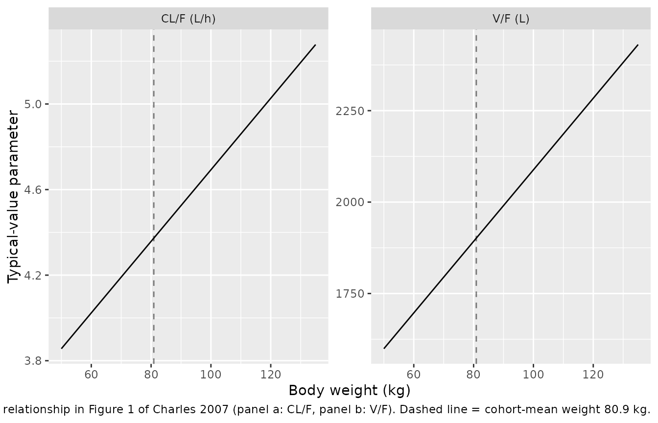

Figure 2 - Visual predictive check after loading and maintenance doses

Charles 2007 Figure 2 shows degenerate VPC plots of plasma tafenoquine versus post-dose time for four sampling windows: (a) week 1 (post third loading dose), (b) week 4, (c) week 8, (d) week 16. Convert ug/mL to ng/mL (x 1000) for direct comparison with the paper.

sim_vpc <- sim |>
  mutate(
    week_panel = case_when(
      time >= 48                  & time <= 48 + 200                  ~ "Week 1 (post loading)",
      time >= 4 * 7 * 24 + 48     & time <= 4 * 7 * 24 + 48  + 200    ~ "Week 4",
      time >= 8 * 7 * 24 + 48     & time <= 8 * 7 * 24 + 48  + 200    ~ "Week 8",
      time >= 16 * 7 * 24 + 48    & time <= 16 * 7 * 24 + 48 + 200    ~ "Week 16",
      TRUE                                                            ~ NA_character_
    ),
    panel_start = case_when(
      week_panel == "Week 1 (post loading)" ~ 48,
      week_panel == "Week 4"  ~ 4  * 7 * 24 + 48,
      week_panel == "Week 8"  ~ 8  * 7 * 24 + 48,
      week_panel == "Week 16" ~ 16 * 7 * 24 + 48,
      TRUE                    ~ NA_real_
    ),
    postdose_h = time - panel_start,
    Cc_ngml    = Cc * 1000
  ) |>
  filter(!is.na(week_panel), postdose_h >= 0, postdose_h <= 200)

vpc <- sim_vpc |>
  group_by(week_panel, postdose_h) |>
  summarise(
    Q05 = quantile(Cc_ngml, 0.05, na.rm = TRUE),
    Q50 = quantile(Cc_ngml, 0.50, na.rm = TRUE),
    Q95 = quantile(Cc_ngml, 0.95, na.rm = TRUE),
    .groups = "drop"
  )

ggplot(vpc, aes(postdose_h, Q50)) +
  geom_ribbon(aes(ymin = Q05, ymax = Q95), alpha = 0.2) +
  geom_line() +
  facet_wrap(~ factor(week_panel,
                      levels = c("Week 1 (post loading)", "Week 4", "Week 8", "Week 16"))) +
  labs(x = "Time post-dose (h)", y = "Plasma tafenoquine (ng/mL)",
       caption = "Replicates Figure 2 of Charles 2007: 50th percentile (solid) and 5th-95th percentile band (shaded) from 100 simulated subjects.")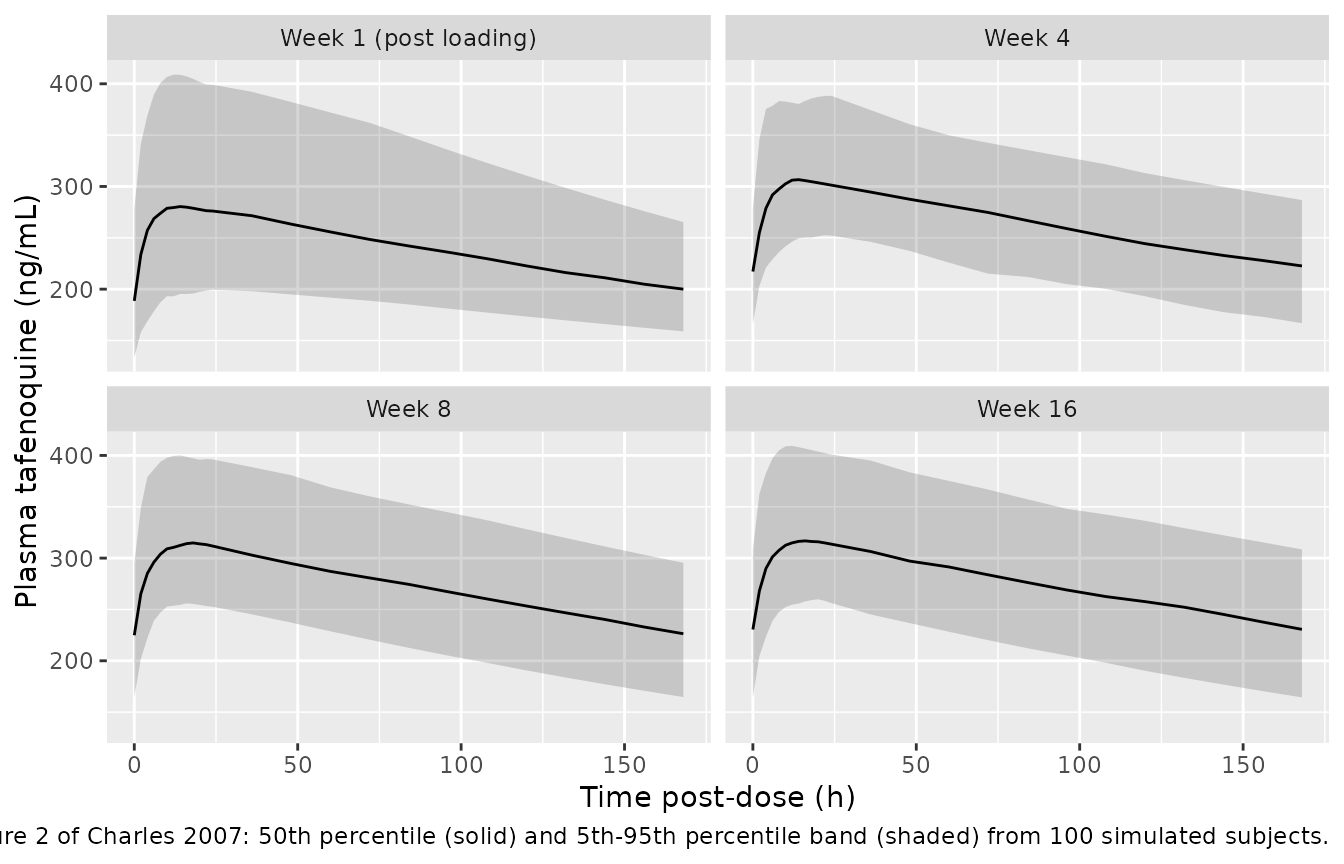

PKNCA validation

NCA is assessed over the week-16 dosing interval (168 h post-dose sampling window) - the last published Figure 2 panel, by which time the profile is at functional steady state given the ~13-day half-life and weekly dosing. The window matches the trough-sample timing reported in Charles 2007 Results paragraph 4 (n=162 subjects at week 4, 8, 16, drawn within 5% of the 168-h post-dose target).

tau      <- 168                                # hours
start_ss <- 16 * 7 * 24 + 48                   # = 2736 h: time of week-16 dose
end_ss   <- start_ss + tau                     # = 2904 h: 168 h post-dose

# Tag a single "treatment" so the PKNCA formula has a group; this also gives
# the side-by-side comparison table below a clean join key.
sim_nca <- sim |>
  filter(time >= start_ss,
         time <= end_ss) |>
  mutate(treatment = "200 mg PO QW (week 16 interval)",
         Cc_ngml   = Cc * 1000) |>
  select(id, time, Cc = Cc_ngml, treatment)

# The week-16 maintenance dose (subset of all maintenance doses)
dose_df <- tibble(id = cohort$id) |>
  mutate(time      = start_ss,
         amt       = 200,
         treatment = "200 mg PO QW (week 16 interval)")

conc_obj <- PKNCA::PKNCAconc(sim_nca, Cc ~ time | treatment + id,
                             concu = "ng/mL", timeu = "hr")
dose_obj <- PKNCA::PKNCAdose(dose_df, amt ~ time | treatment + id,
                             doseu = "mg")

intervals <- data.frame(
  start   = start_ss,
  end     = end_ss,
  cmax    = TRUE,
  cmin    = TRUE,
  tmax    = TRUE,
  auclast = TRUE,
  cav     = TRUE
)

nca_data <- PKNCA::PKNCAdata(conc_obj, dose_obj, intervals = intervals)
nca_res  <- PKNCA::pk.nca(nca_data)
nca_summary <- summary(nca_res)
knitr::kable(nca_summary,
             caption = paste0(
               "Simulated steady-state NCA over a 168-h dosing interval at ",
               "week 20 (200 mg PO once weekly)."
             ))

Simulated steady-state NCA over a 168-h dosing interval at week 20 (200 mg PO once weekly).
Interval Start	Interval End	treatment	N	AUClast (hr*ng/mL)	Cmax (ng/mL)	Cmin (ng/mL)	Tmax (hr)	Cav (ng/mL)
2736	2904	200 mg PO QW (week 16 interval)	100	45900 [16.7]	319 [14.9]	225 [20.5]	14.0 [4.00, 48.0]	273 [16.7]

Comparison against published NCA

Charles 2007 reports steady-state-equivalent observed concentrations at weeks 4, 8 and 16: peak 321 +/- 63 ng/mL within 5% of the typical Tmax (21.4 h post-dose, 42 subjects across the three weeks), and trough 221 +/- 57 ng/mL within 5% of the 168-h post-dose target (162 subjects across the three weeks). The typical-value t_half is reported as 12.7 +/- 3.0 days.

res_tbl <- as.data.frame(nca_res$result) |>
  group_by(PPTESTCD) |>
  summarise(simulated_median = median(PPORRES, na.rm = TRUE),
            simulated_p05    = quantile(PPORRES, 0.05, na.rm = TRUE),
            simulated_p95    = quantile(PPORRES, 0.95, na.rm = TRUE),
            .groups          = "drop")

# Typical-value half-life from the typical-value CL/F and V/F at 80.9 kg.
typ_clf  <- 3.02  * (1 + 0.448 * 80.9 / 80.9)
typ_vf   <- 1110  * (1 + 0.713 * 80.9 / 80.9)
typ_half <- log(2) * typ_vf / typ_clf  / 24            # days

comparison <- tibble::tibble(
  metric    = c("Peak (ng/mL, ~21 h post-dose)",
                "Trough (ng/mL, 168 h post-dose)",
                "Half-life (days, typical)"),
  published = c("321 +/- 63 (n=42, weeks 4/8/16)",
                "221 +/- 57 (n=162, weeks 4/8/16)",
                "12.7 +/- 3.0"),
  simulated = c(
    sprintf("%.0f (5th-95th %.0f-%.0f) [cmax]",
            res_tbl$simulated_median[res_tbl$PPTESTCD == "cmax"],
            res_tbl$simulated_p05[res_tbl$PPTESTCD == "cmax"],
            res_tbl$simulated_p95[res_tbl$PPTESTCD == "cmax"]),
    sprintf("%.0f (5th-95th %.0f-%.0f) [cmin]",
            res_tbl$simulated_median[res_tbl$PPTESTCD == "cmin"],
            res_tbl$simulated_p05[res_tbl$PPTESTCD == "cmin"],
            res_tbl$simulated_p95[res_tbl$PPTESTCD == "cmin"]),
    sprintf("%.1f", typ_half)
  )
)

knitr::kable(comparison,
             caption = "Side-by-side comparison of simulated steady-state metrics with values reported in Charles 2007 (Results paragraphs 4-5).")

Side-by-side comparison of simulated steady-state metrics with values reported in Charles 2007 (Results paragraphs 4-5).
metric	published	simulated
Peak (ng/mL, ~21 h post-dose)	321 +/- 63 (n=42, weeks 4/8/16)	318 (5th-95th 260-411) [cmax]
Trough (ng/mL, 168 h post-dose)	221 +/- 57 (n=162, weeks 4/8/16)	230 (5th-95th 164-308) [cmin]
Half-life (days, typical)	12.7 +/- 3.0	12.6

Assumptions and deviations

IIV correlation between CL/F and V/F not reported. Charles 2007 (Results paragraph 4) states that a covariance between omega^2(CL/F) and omega^2(V/F) was estimated (OFV decreased from 22,265 to 22,248 versus the diagonal-only model) but the numeric value is not given in Table 2. The packaged model uses independent diagonal IIVs; simulated joint CL/F + V/F distributions will therefore be uncorrelated, and joint exposure metrics (e.g. correlated extremes) will be modestly less extreme than the authors’ final fit. Diagonal CV% values match Table 2.
Inter-occasion variability on CL/F not encoded. Charles 2007 estimates an IOV of 18% CV on CL/F (Table 2) on top of the 18% IIV. Encoding IOV would require an OCC covariate column and an occasion-multiplexed eta; packaged simulations therefore underestimate the total within-subject between-occasion spread. Same convention as Hodiamont_2017_gentamicin and Ekhart_2008_carboplatin.
Race / Caucasian fraction. 482 of 490 subjects (98.4%) were Caucasian (Charles 2007 Results paragraph 1); race was not screened as a covariate and is not encoded in the model. The virtual cohort above uses the cohort-mean WT and SD without stratifying by race.
Sex. 14 of 490 subjects (2.9%) were female. Sex on CL/F (delta-OFV = -3) and V/F (delta-OFV = -12) was screened but not retained in the final model (Table 1 models 7-8); the virtual cohort treats subjects as exchangeable.
AGE, CRCL, phospholipidosis. Documented in covariatesDataExcluded for source-trace completeness; none retained in the final model.
Concentration units. Charles 2007 reports concentrations in ng/mL; the model uses ug/mL (= mg/L) to align with the rest of nlmixr2lib. Conversion factor: 1 ug/mL = 1000 ng/mL.
Sampling and dosing windows. The simulation uses the post-third loading dose + weekly maintenance through week 20 - long enough to cover the published Figure 2 panels (week 1 post-loading + weeks 4/8/16 maintenance). The trial ran for 6 months (~26 weeks); steady-state NCA here uses the week-20 interval, which is functionally at steady state given the ~13-day half-life.