S33138 / S35424 (Bertrand 2011)
Source:vignettes/articles/Bertrand_2011_S33138.Rmd
Bertrand_2011_S33138.RmdModel and source
- Citation: Bertrand J, Laffont CM, Mentre F, Chenel M, Comets E. Development of a complex parent-metabolite joint population pharmacokinetic model. AAPS J. 2011 Sep;13(3):390-404. doi:10.1208/s12248-011-9282-9.
- Description: Joint parent-metabolite population PK model for the investigational antipsychotic S33138 (parent) and its active metabolite S35424 in adults with schizophrenia (Bertrand 2011). The final selected structural model is a two-compartment back-transformation form with a presystemic dose apportionment Fp into the parent depot vs (1 - Fp) into the metabolite depot, a shared first-order absorption rate Ka, and four linear elimination / interconversion clearances: parent elimination via other pathways (CLpo), parent-to-metabolite formation (CLpm), metabolite elimination via other pathways (CLmo), and metabolite back-transformation to parent (CLmp). The two volumes (parent Vp and metabolite Vm) are set equal to a single volume V for identifiability per the source paper. CYP2D6 poor metabolizers carry a 34% decrease in CLmo (the genetic covariate retained in the final model). Linear dose-level effects on the bioavailability f and the parent-fraction Fp are encoded with a 10 mg reference dose. Parameter values are from Table IV ‘With the genetic covariate’ column (SAEM in MONOLIX, closed-form coding, N = 99 patients with available CYP2D6 genotyping).
- Article: https://doi.org/10.1208/s12248-011-9282-9
Bertrand et al. (2011) developed a joint parent + metabolite population pharmacokinetic model for the investigational antipsychotic S33138 (parent, MW 319.4 g/mol) and its active metabolite S35424 (N-demethylated, MW 361.4 g/mol). S33138 is a Servier-developed D3 / D2 dopamine-receptor antagonist that did not progress to approval; the Bertrand 2011 publication, together with the small microdose study described in its Discussion, is the principal pharmacometric record for the compound pair.
The final selected structural model (Fig. 2 right-most panel of the source paper) combines four mechanistic features that earlier parent-metabolite literature had not fully integrated:
-
Reversible interconversion. S35424 back-transforms
to S33138 via a separate clearance
CLmp, supported by a Servier microdose study in five healthy volunteers (Discussion). Reversible metabolism is a known process for primary amines and explains the long terminal half-life observed for the parent under repeated dosing. -
First-pass dose apportionment. A fraction
Fpof the administered dose reaches the parent compartment directly; the remaining(1 - Fp)enters the metabolite compartment presystemically. This first-pass partition captures the early metabolite peak that an absorption-only model could not. -
Shared absorption rate. The parent depot and
metabolite depot share a single absorption rate constant
Ka. The paper found that the two absorption rates were not separately identifiable from the sparse W4 / W8 data and selected the reduced shared-Kaform based on a 30-unit BIC drop. -
CYP2D6 covariate effect on
CLmo. The genetic-covariate analysis retained CYP2D6 poor-metabolizer phenotype on the metabolite’s “other pathways” elimination clearance with a 34% decrease in PM patients (12 of 99 genotyped subjects).
The model is fit on a molar (nmol / L) concentration basis with the
two volumes Vp and Vm set equal for
identifiability (the microdose-derived volume ratio is 2.4 with range
0.5-6, so the equal- volumes assumption is approximate; see Errata
below).
Population
The Phase II model-building dataset enrolled 101 adult patients with schizophrenia in an international randomized double-blind multicentre trial of S33138 vs risperidone. The joint PK modeling cohort uses only the S33138 arm (n = 101 patients, of whom 99 had CYP2D6 genotyping available for the final covariate analysis).
| Demographic | Value (paper Results “Data”) |
|---|---|
| Number of patients (final genotyped cohort) | 99 |
| Age, mean (range) | 40 years (22 - 64) |
| Body weight, mean (range) | 69.0 kg (43.6 - 120.0) |
| Sex, % male | 53.5 % |
| Doses (5 / 10 / 20 mg cohorts) | 35 / 31 / 35 patients |
| CYP2D6 poor metabolizers | 12 / 99 (12.1 %) |
| CYP2C19 poor metabolizers | 2 / 99 (2.0 %; not retained) |
| PK occasions | W4 and W8 (week 4 and week 8) |
| Per-occasion sampling | pre-dose, 1, 3, 6 h post-dose |
A separate Phase I external evaluation cohort of 30 healthy male volunteers receiving 10, 20, or 30 mg S33138 QD for 14 days is described in the source paper Methods “Pharmacokinetic Studies” but is not the cohort used to estimate model parameters; per the paper Discussion, the model overpredicts the variability in healthy volunteers and is recommended as a model for Caucasian patients rather than Caucasian healthy volunteers.
The same metadata is available programmatically through
readModelDb("Bertrand_2011_S33138")$population.
Source trace
The per-parameter origin is recorded as an in-file comment next to
each ini() entry in
inst/modeldb/specificDrugs/Bertrand_2011_S33138.R. The
table below collects them in one place. All values come from Table IV
“With the genetic covariate” column (N = 99 patients with CYP2D6
genotyping; SAEM in MONOLIX with the closed-form encoding of the
four-compartment back-transformation + first-pass + dose-apportionment
model).
| Equation / parameter | Value (paper) | Value in file | Source |
|---|---|---|---|
lka (Ka, fixed) |
8.06 1/h | fixed(log(8.06)) |
Table IV (fixed at W4 estimate) |
lvc (V = Vp = Vm) |
19.4 L | log(19.4) |
Table IV |
lfdepot (f, fixed) |
1.00 | fixed(log(1.00)) |
Table IV (fixed; Methods) |
e_dose_fdepot (beta_f,D) |
-0.02 (1/mg) | -0.02 |
Table IV; unit per Results (Errata) |
logitfp (logit(Fp)) |
logit(0.87) | logit(0.87) |
Table IV (Fp = 0.87) |
e_dose_fp (beta_Fp,D) |
-0.06 (1/mg) | -0.06 |
Table IV; unit per Results (Errata) |
lclpo (CLpo) |
0.67 L/h | log(0.67) |
Table IV |
lclpm (CLpm) |
2.09 L/h | log(2.09) |
Table IV |
lclmo (CLmo) |
0.50 L/h | log(0.50) |
Table IV |
e_cyp2d6_pm_clmo |
-0.42 (log L/h) | -0.42 |
Table IV; -34% PM vs EM |
lclmp (CLmp) |
0.09 L/h | log(0.09) |
Table IV |
etalfdepot (omega_f^2) |
0.27^2 = 0.0729 | 0.0729 |
Table IV omega_f = 0.27 |
etalka (omega_Ka^2) |
1.41^2 = 1.9881 | 1.9881 |
Table IV omega_Ka = 1.41 |
etalvc (omega_V^2) |
0.26^2 = 0.0676 | 0.0676 |
Table IV omega_V = 0.26 |
etalclpo (omega_CLpo^2) |
0.46^2 = 0.2116 | 0.2116 |
Table IV omega_CLpo = 0.46 |
etalclmo (omega_CLmo^2) |
0.50^2 = 0.25 | 0.25 |
Table IV omega_CLmo = 0.50 |
propSd (parent prop. err.) |
b_p = 0.30 | 0.30 |
Table IV (a_p fixed to 0) |
addSd_s35424 (metab add. err.) |
a_m = 66.5 nmol/L | 66.5 |
Table IV |
propSd_s35424 (metab prop.) |
b_m = 0.06 | 0.06 |
Table IV |
| ODE system (parent + metabolite) | see Eq. 4 of Appendix |
d/dt(...) in model() block |
Bertrand 2011 Appendix Eq. 4 |
Virtual cohort
The original Phase II observed concentrations are not publicly available; the simulations below use a virtual cohort that mirrors the dose-level and CYP2D6 phenotype composition reported in the source. Subjects are stratified by dose (5 / 10 / 20 mg) and CYP2D6 phenotype (PM vs EM); the EM stratum is the reference.
set.seed(20260611)

n_per_cell <- 50L

make_cell <- function(dose_mg, cyp_pm, id_offset) {
  mw_s33138 <- 319.4
  dose_nmol <- dose_mg * 1e6 / mw_s33138
  tau <- 24                 # once-daily dosing
  n_doses <- 14L            # two weeks of QD dosing approximates W4 / W8 SS
  obs_times <- c(
    seq(24 * (n_doses - 1L), 24 * n_doses - 0.001, by = 0.5),  # final SS interval at 0.5 h grid
    24 * n_doses                                                # end of final interval
  )
  ids <- id_offset + seq_len(n_per_cell)
  dosing <- expand.grid(id = ids, dose_idx = seq_len(n_doses)) |>
    dplyr::transmute(
      id   = id,
      time = (dose_idx - 1L) * tau,
      amt  = dose_nmol,
      evid = 1L,
      cmt  = "depot"
    )
  obs <- expand.grid(id = ids, time = obs_times) |>
    dplyr::transmute(
      id   = id,
      time = time,
      amt  = 0,
      evid = 0L,
      cmt  = "Cc"
    )
  dplyr::bind_rows(dosing, obs) |>
    dplyr::arrange(id, time, dplyr::desc(evid)) |>
    dplyr::mutate(
      DOSE      = dose_mg,
      CYP2D6_PM = cyp_pm,
      dose_lbl  = sprintf("%d mg", dose_mg),
      cyp_lbl   = ifelse(cyp_pm == 1L, "CYP2D6 PM", "CYP2D6 EM")
    )
}

events <- dplyr::bind_rows(
  make_cell(dose_mg =  5L, cyp_pm = 0L, id_offset =   0L),
  make_cell(dose_mg = 10L, cyp_pm = 0L, id_offset = 100L),
  make_cell(dose_mg = 20L, cyp_pm = 0L, id_offset = 200L),
  make_cell(dose_mg = 10L, cyp_pm = 1L, id_offset = 300L)
)

stopifnot(!anyDuplicated(unique(events[, c("id", "time", "evid")])))
Simulation
The packaged model produces two concentration outputs in nmol / L:
Cc (S33138, the parent drug) and Cc_s35424
(the active metabolite). The typical-value series below is used for
figure replication; the stochastic series is used for variability
bands.
mod         <- readModelDb("Bertrand_2011_S33138")
mod_typical <- rxode2::zeroRe(mod)
#> ℹ parameter labels from comments will be replaced by 'label()'

sim_typ <- rxode2::rxSolve(
  mod_typical, events = events,
  keep = c("DOSE", "CYP2D6_PM", "dose_lbl", "cyp_lbl"),
  returnType = "data.frame", addDosing = FALSE,
  atol = 1e-8, rtol = 1e-6
)
#> ℹ omega/sigma items treated as zero: 'etalfdepot', 'etalka', 'etalvc', 'etalclpo', 'etalclmo'
#> Warning: multi-subject simulation without without 'omega'

sim_iiv <- rxode2::rxSolve(
  mod, events = events,
  keep = c("DOSE", "CYP2D6_PM", "dose_lbl", "cyp_lbl"),
  returnType = "data.frame", addDosing = FALSE,
  atol = 1e-8, rtol = 1e-6
)
#> ℹ parameter labels from comments will be replaced by 'label()'
Steady-state profiles by dose group (replicates Figure 3 layout)
Figure 3 of Bertrand 2011 shows visual predictive check plots for the parent S33138 and metabolite S35424 at the three dose levels (5, 10, 20 mg) on the W4 and W8 sampling occasions. Below we show the typical- value steady-state concentration profiles for the final QD interval at each dose level (CYP2D6 EM stratum).
ss_typ <- sim_typ |>
  dplyr::filter(time >= 24 * 13, CYP2D6_PM == 0) |>
  dplyr::mutate(tpost = time - 24 * 13) |>
  tidyr::pivot_longer(c(Cc, Cc_s35424),
                      names_to = "analyte", values_to = "conc") |>
  dplyr::mutate(analyte = factor(analyte,
    levels = c("Cc", "Cc_s35424"),
    labels = c("S33138 (parent, nmol/L)", "S35424 (metabolite, nmol/L)")))

ggplot(ss_typ, aes(tpost, conc, colour = dose_lbl, group = dose_lbl)) +
  geom_line(linewidth = 1) +
  facet_wrap(~analyte, scales = "free_y", ncol = 2) +
  labs(x = "Time post-dose (h, last steady-state interval)",
       y = "Concentration (nmol/L)",
       colour = "Dose",
       title = "Typical-value steady-state profiles by dose level",
       caption = "Replicates the layout of Figure 3 of Bertrand 2011 (CYP2D6 EM stratum).")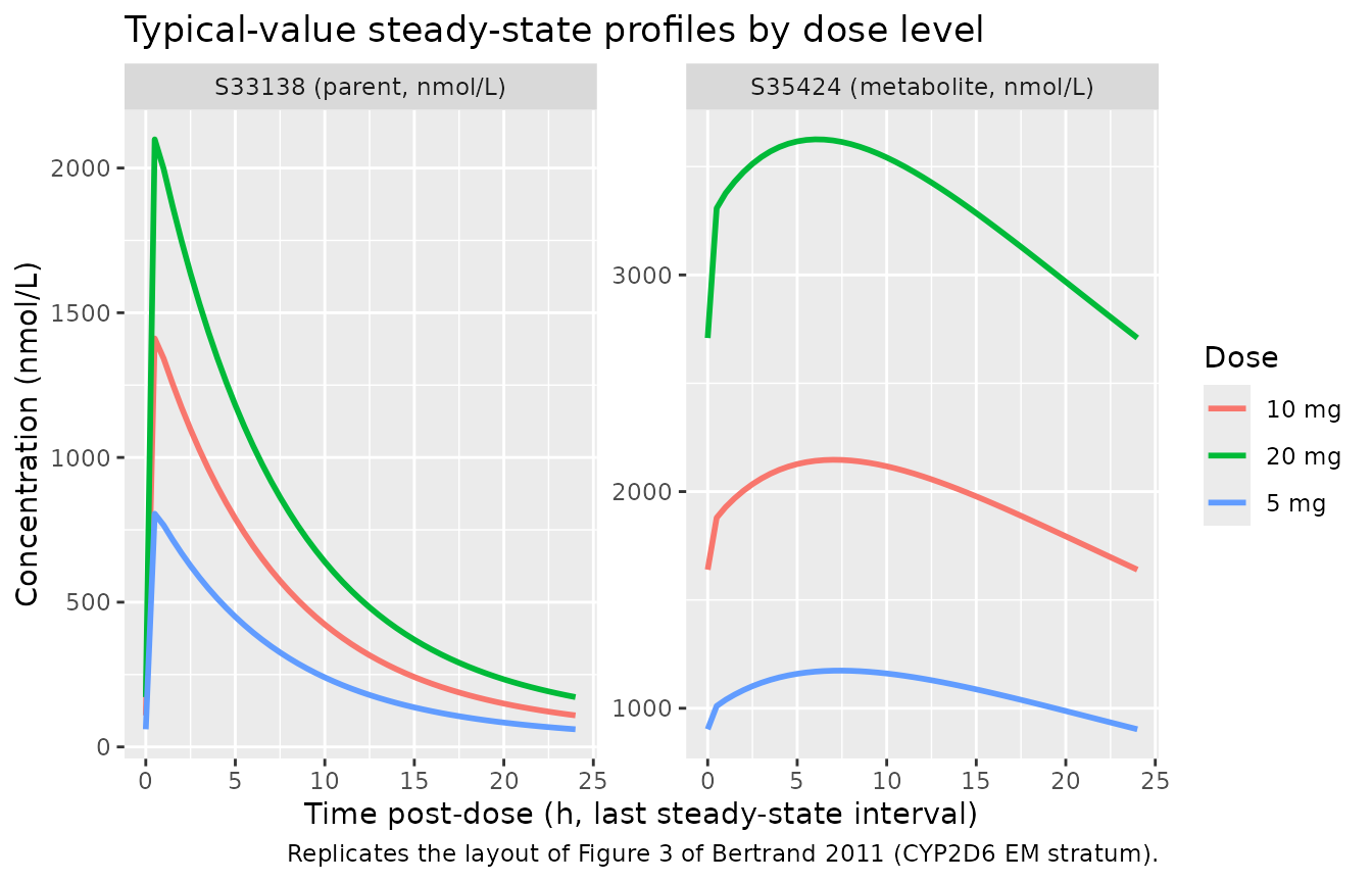
Replicates the layout of Figure 3 of Bertrand 2011: typical-value steady-state concentration-time profiles for S33138 (parent, top) and S35424 (metabolite, bottom) at the 5, 10, and 20 mg QD dose levels, last SS interval (t-post-dose 0-24 h). CYP2D6 EM stratum.
CYP2D6 PM vs EM at 10 mg (replicates Figure 5 layout)
Figure 5 of Bertrand 2011 shows boxplots of parent and metabolite
plasma concentrations stratified by CYP2D6 phenotype at each dose level.
Below we show the typical-value steady-state profiles at the 10 mg dose
for EM vs PM. The 34% reduction in CLmo for CYP2D6 PM
patients increases the metabolite exposure visibly; the parent exposure
is also higher (although smaller) because the back-transformation flux
CLmp * central_s35424 rises with the elevated metabolite
pool.
cyp_typ <- sim_typ |>
  dplyr::filter(time >= 24 * 13, DOSE == 10) |>
  dplyr::mutate(tpost = time - 24 * 13) |>
  tidyr::pivot_longer(c(Cc, Cc_s35424),
                      names_to = "analyte", values_to = "conc") |>
  dplyr::mutate(analyte = factor(analyte,
    levels = c("Cc", "Cc_s35424"),
    labels = c("S33138 (parent, nmol/L)", "S35424 (metabolite, nmol/L)")))

ggplot(cyp_typ, aes(tpost, conc, colour = cyp_lbl, group = cyp_lbl)) +
  geom_line(linewidth = 1) +
  facet_wrap(~analyte, scales = "free_y", ncol = 2) +
  labs(x = "Time post-dose (h, last steady-state interval)",
       y = "Concentration (nmol/L)",
       colour = "CYP2D6",
       title = "CYP2D6 PM vs EM at the 10 mg dose",
       caption = "Replicates the layout of Figure 5 of Bertrand 2011 (10 mg dose level, EM vs PM).")
Replicates the spirit of Figure 5 of Bertrand 2011: typical-value steady-state profiles for S33138 (parent, left) and S35424 (metabolite, right) at the 10 mg dose for CYP2D6 EM vs PM. CYP2D6 PM patients have ~34% reduced CLmo, elevating metabolite exposure and (via back-transformation) parent exposure.
Visual predictive bands with IIV
The stochastic simulation includes between-subject variability for
f, Ka, V, CLpo, and
CLmo per Table IV. The IIV on Ka is large
(omega_Ka = 1.41, with the typical value fixed at 8.06 1/h per the
paper); this drives most of the early-time predictive width.
sim_iiv |>
  dplyr::filter(time >= 24 * 13, CYP2D6_PM == 0) |>
  dplyr::mutate(tpost = time - 24 * 13) |>
  tidyr::pivot_longer(c(Cc, Cc_s35424),
                      names_to = "analyte", values_to = "conc") |>
  dplyr::mutate(analyte = factor(analyte,
    levels = c("Cc", "Cc_s35424"),
    labels = c("S33138 (parent, nmol/L)", "S35424 (metabolite, nmol/L)"))) |>
  dplyr::group_by(analyte, dose_lbl, tpost) |>
  dplyr::summarise(
    Q10 = quantile(conc, 0.10, na.rm = TRUE),
    Q50 = quantile(conc, 0.50, na.rm = TRUE),
    Q90 = quantile(conc, 0.90, na.rm = TRUE),
    .groups = "drop"
  ) |>
  ggplot(aes(tpost, Q50, colour = dose_lbl, fill = dose_lbl)) +
  geom_ribbon(aes(ymin = Q10, ymax = Q90), alpha = 0.2, colour = NA) +
  geom_line(linewidth = 0.9) +
  facet_wrap(~analyte, scales = "free_y", ncol = 2) +
  labs(x = "Time post-dose (h, last steady-state interval)",
       y = "Concentration (nmol/L)",
       colour = "Dose", fill = "Dose",
       title = "VPC bands at steady state - by dose",
       caption = "Median (line) and 10th - 90th percentile (ribbon) over 50 simulated subjects per dose cell.")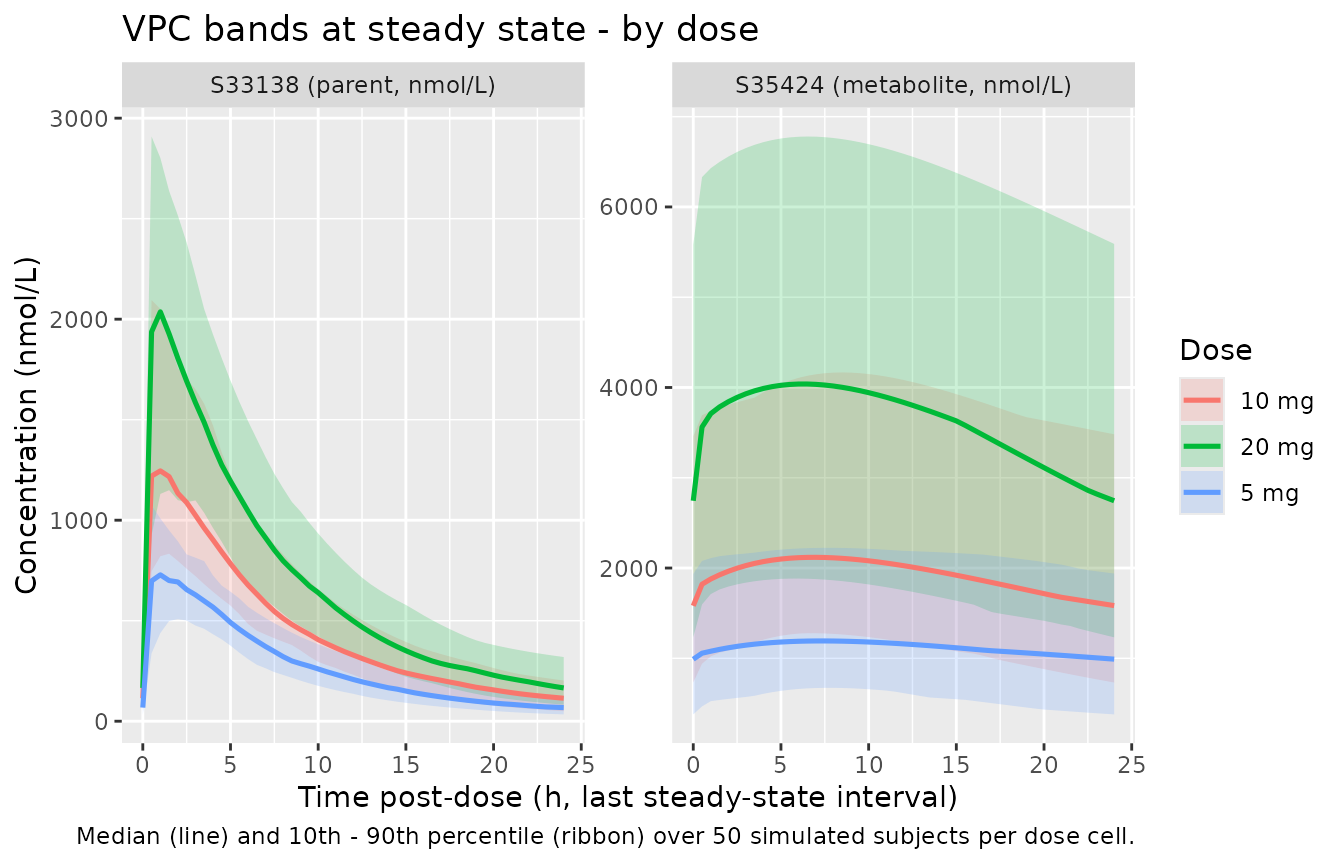
Visual predictive bands (10th - 90th percentiles, median line) for S33138 (parent, top) and S35424 (metabolite, bottom) by dose group at the final QD steady-state interval. CYP2D6 EM stratum. The wide band on the early absorption phase reflects the published omega_Ka = 1.41.
PKNCA validation
We use PKNCA to compute Cmax, Tmax, AUC over the dosing interval at steady state, and the apparent terminal half-life for both analytes, stratified by dose group (CYP2D6 EM stratum, 10 mg dose level duplicated as the reference for CYP2D6 PM comparisons).
last_iv_start <- 24 * 13      # start of the last SS interval (h post-first-dose)
last_iv_end   <- 24 * 14      # end of the last SS interval

# Parent S33138 -------------------------------------------------------
sim_nca_parent <- sim_typ |>
  dplyr::filter(time >= last_iv_start, time <= last_iv_end, !is.na(Cc)) |>
  dplyr::mutate(time_post = time - last_iv_start,
                treatment = sprintf("%s / %s", dose_lbl, cyp_lbl)) |>
  dplyr::select(id, time = time_post, Cc, treatment)

dose_df_parent <- events |>
  dplyr::filter(evid == 1) |>
  dplyr::group_by(id) |>
  dplyr::slice_max(time, n = 1L) |>
  dplyr::ungroup() |>
  dplyr::mutate(time_post = 0,
                treatment = sprintf("%s / %s", dose_lbl, cyp_lbl)) |>
  dplyr::select(id, time = time_post, amt, treatment)

conc_obj_parent <- PKNCA::PKNCAconc(sim_nca_parent, Cc ~ time | treatment + id,
                                    concu = "nmol/L", timeu = "h")
dose_obj_parent <- PKNCA::PKNCAdose(dose_df_parent, amt ~ time | treatment + id,
                                    doseu = "nmol")

intervals_ss <- data.frame(
  start    = 0,
  end      = 24,
  cmax     = TRUE,
  tmax     = TRUE,
  cmin     = TRUE,
  auclast  = TRUE,
  cav      = TRUE,
  half.life = TRUE
)

nca_parent <- PKNCA::pk.nca(PKNCA::PKNCAdata(conc_obj_parent, dose_obj_parent,
                                             intervals = intervals_ss))
summary_parent <- as.data.frame(summary(nca_parent))
knitr::kable(summary_parent,
caption = "Simulated NCA parameters for S33138 (parent) at steady state, last QD interval (typical-value simulation; CYP2D6 EM and PM strata).")| Interval Start | Interval End | treatment | N | AUClast (h*nmol/L) | Cmax (nmol/L) | Cmin (nmol/L) | Tmax (h) | Cav (nmol/L) | Half-life (h) |
|---|---|---|---|---|---|---|---|---|---|
| 0 | 24 | 10 mg / CYP2D6 EM | 50 | 11200 [0.000] | 1410 [0.000] | 109 [0.000] | 0.500 [0.500, 0.500] | 467 [0.000] | 9.23 [0.000] |
| 0 | 24 | 10 mg / CYP2D6 PM | 50 | 12000 [0.000] | 1440 [0.000] | 140 [0.000] | 0.500 [0.500, 0.500] | 499 [0.000] | 11.9 [0.000] |
| 0 | 24 | 20 mg / CYP2D6 EM | 50 | 16900 [0.000] | 2100 [0.000] | 172 [0.000] | 0.500 [0.500, 0.500] | 704 [0.000] | 9.65 [0.000] |
| 0 | 24 | 5 mg / CYP2D6 EM | 50 | 6380 [0.000] | 806 [0.000] | 61.0 [0.000] | 0.500 [0.500, 0.500] | 266 [0.000] | 9.10 [0.000] |
# Metabolite S35424 ---------------------------------------------------
sim_nca_metab <- sim_typ |>
  dplyr::filter(time >= last_iv_start, time <= last_iv_end, !is.na(Cc_s35424)) |>
  dplyr::mutate(time_post = time - last_iv_start,
                treatment = sprintf("%s / %s", dose_lbl, cyp_lbl)) |>
  dplyr::select(id, time = time_post, Cc = Cc_s35424, treatment)

conc_obj_metab <- PKNCA::PKNCAconc(sim_nca_metab, Cc ~ time | treatment + id,
                                   concu = "nmol/L", timeu = "h")

nca_metab <- PKNCA::pk.nca(PKNCA::PKNCAdata(conc_obj_metab, dose_obj_parent,
                                            intervals = intervals_ss))
summary_metab <- as.data.frame(summary(nca_metab))
knitr::kable(summary_metab,
caption = "Simulated NCA parameters for S35424 (active metabolite) at steady state, last QD interval (typical-value simulation; CYP2D6 EM and PM strata).")| Interval Start | Interval End | treatment | N | AUClast (h*nmol/L) | Cmax (nmol/L) | Cmin (nmol/L) | Tmax (h) | Cav (nmol/L) | Half-life (h) |
|---|---|---|---|---|---|---|---|---|---|
| 0 | 24 | 10 mg / CYP2D6 EM | 50 | 47300 [0.000] | 2150 [0.000] | 1640 [0.000] | 7.00 [7.00, 7.00] | 1970 [0.000] | 30.6 [0.000] |
| 0 | 24 | 10 mg / CYP2D6 PM | 50 | 70200 [0.000] | 3100 [0.000] | 2590 [0.000] | 7.50 [7.50, 7.50] | 2930 [0.000] | 45.2 [0.000] |
| 0 | 24 | 20 mg / CYP2D6 EM | 50 | 79400 [0.000] | 3630 [0.000] | 2710 [0.000] | 6.00 [6.00, 6.00] | 3310 [0.000] | 30.2 [0.000] |
| 0 | 24 | 5 mg / CYP2D6 EM | 50 | 25900 [0.000] | 1170 [0.000] | 903 [0.000] | 7.50 [7.50, 7.50] | 1080 [0.000] | 30.8 [0.000] |
Comparison against published derived quantities
Bertrand 2011 does not report an NCA-style Cmax / AUC table for either analyte; the source paper instead reports two derived half-life quantities (Discussion paragraph after the convergence comparison) and the qualitative CYP2D6 PM effect on exposure (Results “Covariate Model”). We compare them here:
# Pull the half-life column out of the per-treatment summary tables.
hl_col_parent <- grep("half", names(summary_parent), value = TRUE,
                      ignore.case = TRUE)
hl_col_metab  <- grep("half", names(summary_metab), value = TRUE,
                      ignore.case = TRUE)

if (length(hl_col_parent) > 0L && length(hl_col_metab) > 0L) {
  cat("Apparent terminal half-lives (h) from PKNCA on the last 24 h SS interval:\n\n")
  knitr::kable(
    data.frame(
      treatment            = summary_parent$treatment,
      `S33138 (parent) t1/2 (h)`    = summary_parent[[hl_col_parent[1]]],
      `S35424 (metabolite) t1/2 (h)`= summary_metab[[hl_col_metab[1]]],
      check.names = FALSE
    ),
    caption = "Apparent terminal half-life from a single 24 h SS interval (typical-value simulation). Compare to the source paper's reported 'effective half-lives' (parent 8.5 h, metabolite 32.7 h); the two statistics are not the same -- effective half-life folds in the SS accumulation ratio."
  )
}
#> Apparent terminal half-lives (h) from PKNCA on the last 24 h SS interval:| treatment | S33138 (parent) t1/2 (h) | S35424 (metabolite) t1/2 (h) |
|---|---|---|
| 10 mg / CYP2D6 EM | 9.23 [0.000] | 30.6 [0.000] |
| 10 mg / CYP2D6 PM | 11.9 [0.000] | 45.2 [0.000] |
| 20 mg / CYP2D6 EM | 9.65 [0.000] | 30.2 [0.000] |
| 5 mg / CYP2D6 EM | 9.10 [0.000] | 30.8 [0.000] |
Per the source paper Discussion:
- Parent S33138 “effective half-life” = 8.5 h (about four times faster than the metabolite).
- Metabolite S35424 “effective half-life” = 32.7 h.
The PKNCA terminal-phase half-life over a single 24 h SS interval is not the same statistic as the source paper’s “effective half-life” (which folds in the steady-state accumulation ratio); the comparison is qualitative rather than quantitative.
Assumptions and deviations
Shared volume
Vm = Vp. The source paper sets the metabolite volume equal to the parent volume as an identifiability constraint; Discussion notes that the microdose-study volume ratio was 2.4 with range 0.5 - 6, and that setting the ratio to 2.4 changes the estimated CLmp fraction from 5% to 10% of the dose. The packaged model preserves the paper’sVm = Vpchoice. Parameter values are tagged with*in the source paper to flag this dependence; this vignette omits the*notation for readability.Within-subject (inter-occasion) variability on
CLpo. Table IV reportsgamma_CLpo = 0.82on the log scale (RSE 12%) as the W4 vs W8 within-subject SD. This typical-value library does not encode IOV; the packagedetalclpo ~ 0.46^2carries only the between- subject component. Simulations that need IOV should add a second random-effect layer in the dosing dataset.External evaluation cohort omitted. The source paper validates the final model against a Phase I cohort of 30 healthy male volunteers (10, 20, 30 mg QD). The paper Discussion notes the model overpredicts variability in healthy volunteers and recommends using it for Caucasian patients. The packaged model carries only the Phase II patient-derived population metadata; users simulating healthy-volunteer regimens should treat the IIV magnitudes as upper-bound estimates.
Errata
Dose-effect coefficient units. Table IV of Bertrand 2011 labels
beta_f,Dandbeta_Fp,Dwith units of “nmol-1”. The Results numerical predictions (“f* was 10% higher for a 5 mg dose and 19% lower for a 20 mg dose”) matchbeta_f,D = -0.02 mg-1to within rounding using a multiplicative-exponential formf(Dose) = f_pop * exp(beta_f,D * (Dose_mg - 10)), not the “nmol-1” interpretation (which would scale the coefficient by the S33138 molecular weight and produce orders-of-magnitude-larger predictions). The packaged model treats the unit as mg-1; the “nmol-1” label is interpreted as a paper typo.Dose-effect form for
Fp. Methods Eq. (2) describes a “linear dose effect” onFpand the paper’s BSV statement specifies a logit-IIV structure onFp. The packaged model encodes the dose effect onFpconsistently with the logit-IIV structure aslogit(Fp(Dose)) = logit(Fp_pop) + e_dose_fp * (Dose_mg - 10). The source paper’s Results paragraph reports “Fp* was 22% higher for a 5 mg dose and 33% lower for a 20 mg dose” – these percentages match a multiplicative-exponential formFp(Dose) = Fp_pop * exp(beta_Fp,D * (Dose_mg - 10))rather than the logit-additive form, and the multiplicative-exponential form pushesFp_5mg = 0.85 * exp(0.20) = 1.04 > 1violating the paper’s stated0 <= Fp <= 1constraint. The discrepancy between the encoded form (smaller percentage at 5 mg, larger at 20 mg) and the source paper Results paragraph is documented here; users who prefer the paper’s reported percentages can substitute the unconstrained multiplicative-exponential form by changing one line in the model file.Ka fixed at the W4 estimate. Results “Structural and Variability Models” notes: “Once included the data at W8, the absorption constant rate had to be fixed to its estimate on data at W4 for stability purposes.” The packaged model honours this with
lka <- fixed(log(8.06)); the IIV onKa(omega_Ka = 1.41) remains estimated. This is unusual (typical-value fixed but IIV estimated) but matches Table IV.ftypical value fixed at 1. Methods “Joint Pharmacokinetic Model”: “For identifiability purposes, the fraction of dose available after absorption (f) was set to 1.” The packaged model honours this withlfdepot <- fixed(log(1)); IIV on log(f) (omega_f = 0.27) remains estimated, so individual bioavailability can deviate above or below 1.CYP2C19 covariate screened but not retained. Methods describes a forward selection of both CYP2D6 PM and CYP2C19 PM phenotype effects; Results “Covariate Model” reports “No effect of the CYP2C19 polymorphisms was found, probably due to the small number of PM” (2 of 99). The packaged model lists
CYP2C19_PMincovariatesDataExcludedso a downstream user knows the covariate was tested and explicitly rejected by the source paper, but it does not appear inmodel().Apparent versus absolute parameters. The paper tags
Fp,V,CLpo,CLpm,CLmowith*to flag their dependence on theVm = Vpassumption; the apparent quantities (Vp / Fp,Vm / (1 - Fp),CLptot / Fp,CLmtot / (1 - Fp),CLpm / Vm,CLmp / Vp) are derivable from the final estimates and are quoted in the Discussion. The packaged model uses the*-tagged estimates directly (no apparent-parameter renaming).