Lemborexant (Lalovic 2020)

Model and source

• Citation: Lalovic B, Majid O, Aluri J, Landry I, Moline M, Hussein Z. (2020). Population Pharmacokinetics and Exposure-Response Analyses for the Most Frequent Adverse Events Following Treatment With Lemborexant, an Orexin Receptor Antagonist, in Subjects With Insomnia Disorder. Journal of Clinical Pharmacology 60(12):1642-1654. doi:10.1002/jcph.1683.
• Description: Three-compartment population PK model for oral lemborexant (a dual orexin receptor antagonist) in 1892 healthy adults, healthy elderly subjects and adults and elderly subjects with insomnia disorder, pooled from 12 phase 1-3 studies (Lalovic 2020). Absorption is sequential: a zero-order release of duration D1 into the depot after an absorption lag, followed by first-order absorption (ka) into the central compartment; elimination is linear from central. Apparent clearance (CL/F) decreases with body mass index (power, referenced to 25 kg/m^2), with alkaline phosphatase (power, referenced to 71 U/L) and is 26% lower in the elderly (> 65 years). The absorption effects – tablet versus capsule and bedtime dosing on D1, tablet and a high-fat meal on ka, and a high-fat meal on relative bioavailability – were estimated on the extensively sampled phase 1 data and FIXED in the final model, as were ka, D1, the lag time and the IIV on D1, ka and F1. Diagonal IIV on CL/F, Vc/F, Q/F, Vp/F, Q2/F, Vp2/F, D1, ka and F1. Combined additive + proportional residual error with separate parameter pairs for samples taken up to 3 h after the dose and later than 3 h after the dose. Companion landmark exposure-response models for six treatment-emergent adverse events are packaged as Lalovic_2020_lemborexant_.
• Article (open access): https://doi.org/10.1002/jcph.1683
• Supplemental information (Supplemental Tables S1-S2, Figures S1-S4): https://doi.org/10.1002/jcph.1683

Lemborexant is a dual orexin receptor antagonist approved for the treatment of insomnia. Lalovic 2020 reports two analyses, and this package carries both:

• a population PK model built on 12 230 concentrations from 1892 subjects in 12 phase 1-3 studies – Lalovic_2020_lemborexant; and
• exposure-response models for the six most frequent treatment-emergent adverse events (TEAEs) in studies 202, 303 (SUNRISE 2) and 304 (SUNRISE 1), each a logistic regression on the individual average steady-state concentration (Cav,ss) – Lalovic_2020_lemborexant_somnolence, _nasopharyngitis, _uti (urinary tract infection), _influenza, _urti (upper respiratory tract infection) and _headache.

The six adverse-event regressions were fitted independently, so each is its own model file. The paper prints no regression coefficients for them: it tabulates the fitted probabilities for a single reference subject (a 75-year-old White woman) in Table 4. The coefficients here were back-solved from that table (see the section on the exposure-response models below).

Population

The PK analysis pooled 6 extensively and 3 sparsely sampled phase 1 studies, 1 phase 2 study and 2 phase 3 studies (Supplemental Table S1). Subjects were 18-88 years old (median 57), weighed 37-168 kg (median 74.1) with a BMI of 14.4-62.1 kg/m^2 (median 26.5), were 66% female and 70% White, and 547 of the 1892 were elderly (Table 1). The phase 1 subjects were healthy adults and healthy elderly subjects; the phase 2 and 3 subjects had insomnia disorder, and study 202 enrolled subjects with irregular sleep-wake rhythm disorder. Early studies used a capsule, later ones the tablet (1755 of 1892 subjects). Doses spanned 1-100 mg; the phase 3 doses were 5 and 10 mg at bedtime.

The exposure-response data set held 1664 subjects from studies 202 (n = 62), 303 (n = 726) and 304 (n = 524), on placebo or 5-15 mg lemborexant.

str(rxode2::rxode(readModelDb("Lalovic_2020_lemborexant"))$population)
#> ℹ parameter labels from comments will be replaced by 'label()'
#> List of 17
#>  $ species         : chr "human"
#>  $ n_subjects      : num 1892
#>  $ n_studies       : num 12
#>  $ n_observations  : num 12230
#>  $ age_range       : chr "18-88 years"
#>  $ age_median      : chr "57 years"
#>  $ weight_range    : chr "37-168 kg"
#>  $ weight_median   : chr "74.1 kg"
#>  $ bmi_range       : chr "14.4-62.1 kg/m^2 (median 26.5)"
#>  $ sex_female_pct  : num 66
#>  $ race_ethnicity  : Named num [1:6] 70.5 17.7 8.2 1.7 0.3 1.6
#>   ..- attr(*, "names")= chr [1:6] "White" "Black or African American" "Japanese" "Other Asian" ...
#>  $ disease_state   : chr "Healthy adults and healthy elderly subjects (phase 1) and adults and elderly subjects with insomnia disorder (p"| __truncated__
#>  $ dose_range      : chr "1-100 mg once daily orally (phase 3: 5 and 10 mg at bedtime)"
#>  $ hepatic_function: chr "ALP median 71 U/L (range 13-256); ALT median 17 U/L; AST median 19 U/L"
#>  $ renal_function  : chr "Creatinine clearance median 97.3 mL/min (range 26.8-319)"
#>  $ co_medication   : chr "Concomitant PPI 112 subjects; weak CYP3A inhibitors 22 subjects"
#>  $ notes           : chr "Demographics from Lalovic 2020 Table 1 (n = 1892). 6 extensively and 3 sparsely sampled phase 1 studies (407 su"| __truncated__

Source trace

Item	Value	Source location
Structure: 3 compartments, linear elimination	depot, central, 2 peripherals	Results, Base Model; Supplemental Figure S2
Absorption: lag, then zero-order (D1) into depot, then first-order (ka)	ADVAN12, D1 on CMT 1	Results, Base Model; Supplemental Figure S2
lcl CL/F	22.7 L/h	Table 2
lvc V2/F	9.09 L	Table 2
lq Q3/F	32.1 L/h	Table 2
lvp V3/F	278 L	Table 2
lq2 Q4/F	31.0 L/h	Table 2
lvp2 V4/F	783 L	Table 2
ld1 D1, capsule	0.467 h (fixed)	Table 2
lka Ka, capsule	0.532 1/h (fixed)	Table 2
ltlag ALAG1	0.403 h (fixed)	Table 2
lfdepot F1	1 (fasted reference)	Table 2 lists only the food effect
e_bmi_cl	-0.428, (BMI/25)^theta	Table 2; reference back-solved (see Assumptions)
e_alp_cl	-0.118, (ALP/71)^theta	Table 2; reference = Table 1 median and Table 3 footnote
e_age_gt65_cl	0.739^elderly	Table 2
e_form_tablet_d1	0.254 (fixed)	Table 2; Results give 0.118 h for the tablet
e_dosetime_evening_d1	2.33 (fixed)	Table 2 ‘D1, nighttime dosing’
e_form_tablet_ka	1.12 (fixed)	Table 2
e_fed_highfat_ka	0.695 (fixed)	Table 2
e_fed_highfat_fdepot	1.21 (fixed)	Table 2
IIV, CL/F V2/F Q3/F V3/F Q4/F V4/F	48.1, 142, 56.8, 82.0, 46.5, 41.4 %CV	Table 2; variance = (CV/100)^2 per the Table 2 abbreviation ‘CV, square root of variance x 100’
IIV, D1 Ka F1 (fixed)	167, 43.8, 68.1 %CV	Table 2
propSd_early, addSd_early (TAD <= 3 h)	0.329, 2.62 ng/mL	Table 2
propSd_late, addSd_late (TAD > 3 h)	0.143, 0.0189 ng/mL	Table 2
Covariate forms: power for continuous, theta^indicator for dichotomous	–	Table 2 footnote
TEAE models: logit_placebo	qlogis(placebo row)	Table 4, Placebo row
TEAE models: logit_active, e_cav_logit	back-solved	Table 4, ten 5 mg and 10 mg rows (see below)

The population PK model

Typical-value profiles

The phase 3 regimen is the tablet taken at bedtime, fasted. For the reference adult (BMI 25 kg/m^2, ALP 71 U/L) that gives D1 = 0.467 x 0.254 x 2.33 = 0.276 h and ka = 0.532 x 1.12 = 0.596 1/h. Every dose record carries rate = -2, which is what makes rxode2 honour the modelled duration dur(depot).

mod <- readModelDb("Lalovic_2020_lemborexant")
mod_typ <- rxode2::zeroRe(mod)
#> ℹ parameter labels from comments will be replaced by 'label()'
#> Warning: No sigma parameters in the model

ref_cov <- data.frame(
  BMI = 25, ALP = 71, AGE_GT65 = 0,
  FORM_TABLET = 1, FED_HIGHFAT = 0, DOSETIME_EVENING = 1
)

# Once-daily dosing for n_days days, observations over one chosen interval.
ss_events <- function(dose, n_days, obs_day, cov, step = 0.05) {
  doses <- data.frame(
    time = 24 * (seq_len(n_days) - 1), amt = dose, evid = 1L,
    rate = -2, cmt = "depot"
  )
  obs <- data.frame(
    time = 24 * (obs_day - 1) + seq(0, 24, by = step), amt = 0, evid = 0L,
    rate = 0, cmt = "central"
  )
  ev <- dplyr::bind_rows(doses, obs) |> dplyr::arrange(time, dplyr::desc(evid))
  ev$id <- 1L
  cbind(ev, cov[rep(1, nrow(ev)), , drop = FALSE])
}

trap <- function(t, y) sum(diff(t) * (utils::head(y, -1) + utils::tail(y, -1)) / 2)

n_days <- 42
s_d1 <- rxode2::rxSolve(mod_typ, ss_events(5, 1, 1, ref_cov), returnType = "data.frame")
#> ℹ omega/sigma items treated as zero: 'etalcl', 'etalvc', 'etalq', 'etalvp', 'etalq2', 'etalvp2', 'etald1', 'etalka', 'etalfdepot'
s_ss <- rxode2::rxSolve(mod_typ, ss_events(5, n_days, n_days, ref_cov), returnType = "data.frame")
#> ℹ omega/sigma items treated as zero: 'etalcl', 'etalvc', 'etalq', 'etalvp', 'etalq2', 'etalvp2', 'etald1', 'etalka', 'etalfdepot'
s_prev <- rxode2::rxSolve(mod_typ, ss_events(5, n_days, n_days - 1, ref_cov), returnType = "data.frame")
#> ℹ omega/sigma items treated as zero: 'etalcl', 'etalvc', 'etalq', 'etalvp', 'etalq2', 'etalvp2', 'etald1', 'etalka', 'etalfdepot'
s_d1 <- s_d1[!is.na(s_d1$Cc), ]
s_ss <- s_ss[!is.na(s_ss$Cc), ]
s_prev <- s_prev[!is.na(s_prev$Cc), ]
t_ss <- s_ss$time - min(s_ss$time)

auc_d1 <- trap(s_d1$time, s_d1$Cc)
auc_ss <- trap(s_ss$time, s_ss$Cc)
auc_prev <- trap(s_prev$time, s_prev$Cc)
cav_ss <- auc_ss / 24

dplyr::bind_rows(
  data.frame(t = s_d1$time, Cc = s_d1$Cc, Profile = "Day 1"),
  data.frame(t = t_ss, Cc = s_ss$Cc, Profile = "Steady state")
) |>
  ggplot2::ggplot(ggplot2::aes(t, Cc, colour = Profile)) +
  ggplot2::geom_line(linewidth = 1) +
  ggplot2::labs(x = "Time after dose (h)", y = "Lemborexant (ng/mL)", colour = NULL) +
  ggplot2::theme_bw()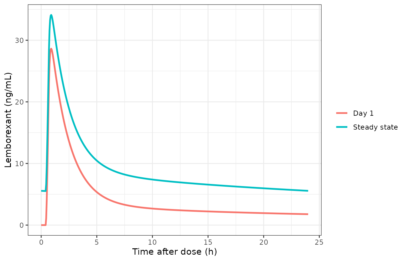

Typical-value lemborexant concentrations after the first 5 mg bedtime tablet dose and at steady state, reference adult (BMI 25 kg/m^2, ALP 71 U/L).

Three checks follow. The first is an identity: at steady state the average concentration must equal F x dose / (24 x CL/F), a statement about the model itself that does not depend on the paper. The other two compare with numbers stated in the Discussion of Lalovic 2020.

cav_closed <- 1000 * 5 / (24 * 22.7) # ng/mL; F = 1 and CL/F = 22.7 L/h at the reference
c_at <- function(h) stats::approx(t_ss, s_ss$Cc, xout = h)$y
cum_auc <- function(h) trap(t_ss[t_ss <= h], s_ss$Cc[t_ss <= h])

typ_tab <- data.frame(
  Quantity = c(
    "Cav,ss (ng/mL), simulated",
    "Cav,ss (ng/mL), dose / (24 x CL/F)",
    "Accumulation ratio AUCtau,ss / AUC0-24 day 1",
    "Fraction of AUCtau,ss eliminated by 8 h",
    "Fraction of AUCtau,ss eliminated by 9 h",
    "Cmax,ss / C(8 h)",
    "Cmax,ss / C(9 h)"
  ),
  Model = c(
    cav_ss, cav_closed, auc_ss / auc_d1, cum_auc(8) / auc_ss,
    cum_auc(9) / auc_ss, max(s_ss$Cc) / c_at(8), max(s_ss$Cc) / c_at(9)
  ),
  Paper = c("--", "--", "1.9", "0.53-0.57", "0.53-0.57", "3.5-4", "3.5-4")
)
typ_tab$Model <- signif(typ_tab$Model, 3)
knitr::kable(typ_tab, caption = "Typical-value checks against the Discussion of Lalovic 2020.")

Typical-value checks against the Discussion of Lalovic 2020.

Quantity	Model	Paper
Cav,ss (ng/mL), simulated	9.180	–
Cav,ss (ng/mL), dose / (24 x CL/F)	9.180	–
Accumulation ratio AUCtau,ss / AUC0-24 day 1	2.010	1.9
Fraction of AUCtau,ss eliminated by 8 h	0.526	0.53-0.57
Fraction of AUCtau,ss eliminated by 9 h	0.561	0.53-0.57
Cmax,ss / C(8 h)	4.270	3.5-4
Cmax,ss / C(9 h)	4.460	3.5-4

stopifnot(
  # Steady state reached: successive intervals agree.
  abs(auc_ss / auc_prev - 1) < 1e-3,
  # Identity: steady-state average concentration = dose / (tau x CL/F).
  abs(cav_ss / cav_closed - 1) < 0.005,
  # Discussion: accumulation ratio 1.9 on once-daily bedtime dosing.
  abs(auc_ss / auc_d1 - 1.9) < 0.2,
  # Discussion: 53%-57% of AUCss eliminated 8-9 h after the dose.
  cum_auc(8) / auc_ss > 0.50, cum_auc(9) / auc_ss < 0.60
)

The model reproduces the accumulation ratio and the fraction of the steady-state AUC gone by the morning. The peak-to-morning ratio comes out at about 4.3-4.5 for the typical subject against the 3.5- to 4-fold quoted “on average”; the paper’s figure is a mean over individuals, and the very large between-subject variability on V2/F (142% CV) and D1 (167% CV) flattens individual peaks, so the typical value sits above the average ratio. It is not used as a gate.

Covariate effects (replicates the Results text and Table 3)

The Results quote the size of each clearance covariate relative to the typical subject. They are closed-form consequences of Table 2 once the reference values are fixed, so they check the transcription and the unprinted BMI reference (25 kg/m^2; see Assumptions).

cl_rel <- function(BMI = 25, ALP = 71, AGE_GT65 = 0) {
  (BMI / 25)^-0.428 * (ALP / 71)^-0.118 * 0.739^AGE_GT65
}
eff <- data.frame(
  Statement = c(
    "Elderly: CL/F lower by", "ALP 150 U/L: exposure higher by",
    "ALP 35 U/L: exposure lower by", "BMI 32: exposure higher by",
    "BMI 40: exposure higher by", "BMI 15: CL/F higher by"
  ),
  Model_pct = 100 * c(
    1 - cl_rel(AGE_GT65 = 1), 1 / cl_rel(ALP = 150) - 1,
    1 - 1 / cl_rel(ALP = 35), 1 / cl_rel(BMI = 32) - 1,
    1 / cl_rel(BMI = 40) - 1, cl_rel(BMI = 15) - 1
  ),
  Paper_pct = c(26, 9, 9, 11, 22, 25)
)
eff$Model_pct <- round(eff$Model_pct, 1)
eff |>
  dplyr::rename(`Results statement` = Statement, `Model (%)` = Model_pct, `Paper (%)` = Paper_pct) |>
  knitr::kable(caption = "Covariate effect sizes quoted in the Results ('Clinically Relevant Covariates').")

Covariate effect sizes quoted in the Results (‘Clinically Relevant Covariates’).

Results statement	Model (%)	Paper (%)
Elderly: CL/F lower by	26.1	26
ALP 150 U/L: exposure higher by	9.2	9
ALP 35 U/L: exposure lower by	8.0	9
BMI 32: exposure higher by	11.1	11
BMI 40: exposure higher by	22.3	22
BMI 15: CL/F higher by	24.4	25

stopifnot(all(abs(eff$Model_pct - eff$Paper_pct) < 1.5))

Table 3 compares steady-state AUC across BMI classes and for overweight elderly versus normal-weight adults at 5 mg nightly, with ALP at its 71 U/L median. The published ratios come from 250 resampled subjects, so the typical-value ratios below are not expected to match to the last percent.

profiles <- data.frame(
  Profile = c("Normal (BMI 22.9)", "Underweight (BMI 17.4)", "Overweight (BMI 27.4)",
              "Obese (BMI 32.7)", "Elderly, overweight (BMI 26.6)"),
  BMI = c(22.9, 17.4, 27.4, 32.7, 26.6),
  AGE_GT65 = c(0, 0, 0, 0, 1),
  Paper = c(NA, 89, 111, 119, 139)
)
profiles$AUCss <- vapply(seq_len(nrow(profiles)), function(i) {
  cv <- ref_cov
  cv$BMI <- profiles$BMI[i]
  cv$AGE_GT65 <- profiles$AGE_GT65[i]
  s <- rxode2::rxSolve(mod_typ, ss_events(5, n_days, n_days, cv), returnType = "data.frame")
  s <- s[!is.na(s$Cc), ]
  trap(s$time, s$Cc)
}, numeric(1))
#> ℹ omega/sigma items treated as zero: 'etalcl', 'etalvc', 'etalq', 'etalvp', 'etalq2', 'etalvp2', 'etald1', 'etalka', 'etalfdepot'
#> ℹ omega/sigma items treated as zero: 'etalcl', 'etalvc', 'etalq', 'etalvp', 'etalq2', 'etalvp2', 'etald1', 'etalka', 'etalfdepot'
#> ℹ omega/sigma items treated as zero: 'etalcl', 'etalvc', 'etalq', 'etalvp', 'etalq2', 'etalvp2', 'etald1', 'etalka', 'etalfdepot'
#> ℹ omega/sigma items treated as zero: 'etalcl', 'etalvc', 'etalq', 'etalvp', 'etalq2', 'etalvp2', 'etald1', 'etalka', 'etalfdepot'
#> ℹ omega/sigma items treated as zero: 'etalcl', 'etalvc', 'etalq', 'etalvp', 'etalq2', 'etalvp2', 'etald1', 'etalka', 'etalfdepot'
profiles$Model <- round(100 * profiles$AUCss / profiles$AUCss[1], 1)
profiles |>
  dplyr::select(Profile, Model, Paper) |>
  dplyr::rename(`Model AUCss ratio (%)` = Model, `Table 3 ratio (%)` = Paper) |>
  knitr::kable(caption = "Replicates Table 3 of Lalovic 2020 (reference: normal-BMI adult).")

Replicates Table 3 of Lalovic 2020 (reference: normal-BMI adult).

Profile	Model AUCss ratio (%)	Table 3 ratio (%)
Normal (BMI 22.9)	100.0	NA
Underweight (BMI 17.4)	88.9	89
Overweight (BMI 27.4)	108.0	111
Obese (BMI 32.7)	116.5	119
Elderly, overweight (BMI 26.6)	144.3	139

chk3 <- profiles[-1, ]
stopifnot(all(abs(chk3$Model / chk3$Paper - 1) < 0.05))

The underweight ratio matches exactly; the overweight and obese ratios fall 2-3 percentage points below the published ones and the elderly-overweight ratio 5 points above (144% against 139%), within 4% in relative terms and the scale expected from resampling 250 subjects.

Stochastic simulation of the phase 3 regimen

A virtual cohort of 200 subjects per arm takes 5 or 10 mg tablets at bedtime, fasted, for 42 days. BMI and ALP are log-normal around the Table 1 medians (26.5 kg/m^2, 71 U/L) with coefficients of variation of 18% and 30% (from the Table 1 SDs), redrawn when outside the Table 1 ranges, and 29% of subjects are elderly (547/1892, Table 1).

set.seed(20201201)
rxode2::rxSetSeed(20201201)
n_per_arm <- 200

draw_in_range <- function(n, median, cv, lo, hi) {
  x <- stats::rlnorm(n, log(median), sqrt(log(1 + cv^2)))
  bad <- x < lo | x > hi
  while (any(bad)) {
    x[bad] <- stats::rlnorm(sum(bad), log(median), sqrt(log(1 + cv^2)))
    bad <- x < lo | x > hi
  }
  x
}

make_cohort <- function(dose, id_offset) {
  n <- n_per_arm
  data.frame(
    id = id_offset + seq_len(n),
    dose = dose,
    treatment = paste(dose, "mg"),
    BMI = draw_in_range(n, 26.5, 0.185, 14.4, 62.1),
    ALP = draw_in_range(n, 71, 0.30, 13, 256),
    AGE_GT65 = stats::rbinom(n, 1, 547 / 1892),
    FORM_TABLET = 1, FED_HIGHFAT = 0, DOSETIME_EVENING = 1
  )
}
cohort <- dplyr::bind_rows(make_cohort(5, 0L), make_cohort(10, n_per_arm))

obs_start <- 24 * (n_days - 1)
dose_rows <- cohort |>
  dplyr::select(id, dose) |>
  tidyr::crossing(day = seq_len(n_days)) |>
  dplyr::transmute(id, time = 24 * (day - 1), amt = dose, evid = 1L, rate = -2, cmt = "depot")
obs_rows <- cohort |>
  dplyr::select(id) |>
  tidyr::crossing(time = obs_start + c(0, 0.25, 0.5, 0.75, 1, 1.5, 2, 3, 4, 6, 8, 9, 12, 16, 20, 24)) |>
  dplyr::mutate(amt = 0, evid = 0L, rate = 0, cmt = "central")
events <- dplyr::bind_rows(dose_rows, obs_rows) |>
  dplyr::left_join(cohort, by = "id") |>
  dplyr::arrange(id, time, dplyr::desc(evid))
stopifnot(!anyDuplicated(cohort$id))

sim <- rxode2::rxSolve(
  mod, events,
  keep = c("treatment", "dose"), returnType = "data.frame"
)
#> ℹ parameter labels from comments will be replaced by 'label()'

sim |>
  dplyr::filter(!is.na(Cc)) |>
  dplyr::mutate(tad = time - obs_start) |>
  dplyr::group_by(treatment, tad) |>
  dplyr::summarise(
    p05 = stats::quantile(Cc, 0.05), p50 = stats::median(Cc), p95 = stats::quantile(Cc, 0.95),
    .groups = "drop"
  ) |>
  ggplot2::ggplot(ggplot2::aes(tad, p50, colour = treatment, fill = treatment)) +
  ggplot2::geom_ribbon(ggplot2::aes(ymin = p05, ymax = p95), alpha = 0.2, colour = NA) +
  ggplot2::geom_line(linewidth = 1) +
  ggplot2::scale_y_log10() +
  ggplot2::labs(x = "Time after dose (h)", y = "Lemborexant (ng/mL)", colour = NULL, fill = NULL) +
  ggplot2::theme_bw()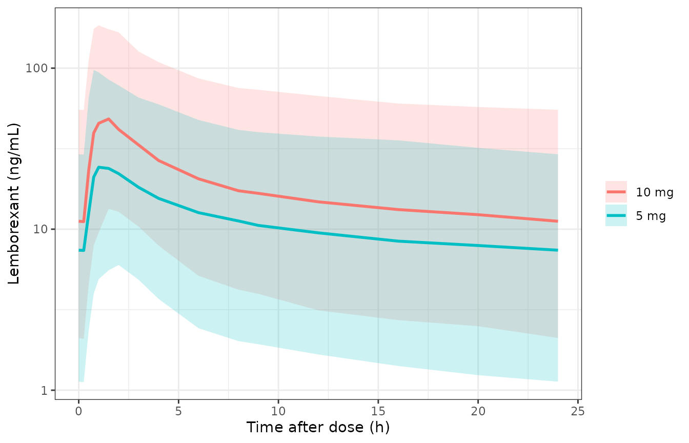

Simulated steady-state lemborexant concentrations (median and 5th-95th percentiles) over the last 24 h dosing interval of 5 and 10 mg at bedtime. Lalovic 2020 Figure 2 shows the corresponding prediction-corrected VPCs stratified by study.

sim |>
  dplyr::distinct(id, .keep_all = TRUE) |>
  dplyr::left_join(dplyr::select(cohort, id, BMI_c = BMI, AGE_c = AGE_GT65), by = "id") |>
  dplyr::mutate(
    Age = ifelse(AGE_c == 1, "Elderly (> 65 y)", "Adult"),
    `BMI class` = cut(BMI_c, c(0, 18.5, 25, 30, Inf), right = FALSE,
                      labels = c("< 18.5", "18.5-24.9", "25-29.9", ">= 30"))
  ) |>
  ggplot2::ggplot(ggplot2::aes(`BMI class`, cl, fill = Age)) +
  ggplot2::geom_boxplot(outlier.size = 0.5) +
  ggplot2::scale_y_log10() +
  ggplot2::labs(y = "Individual CL/F (L/h)", fill = NULL) +
  ggplot2::theme_bw()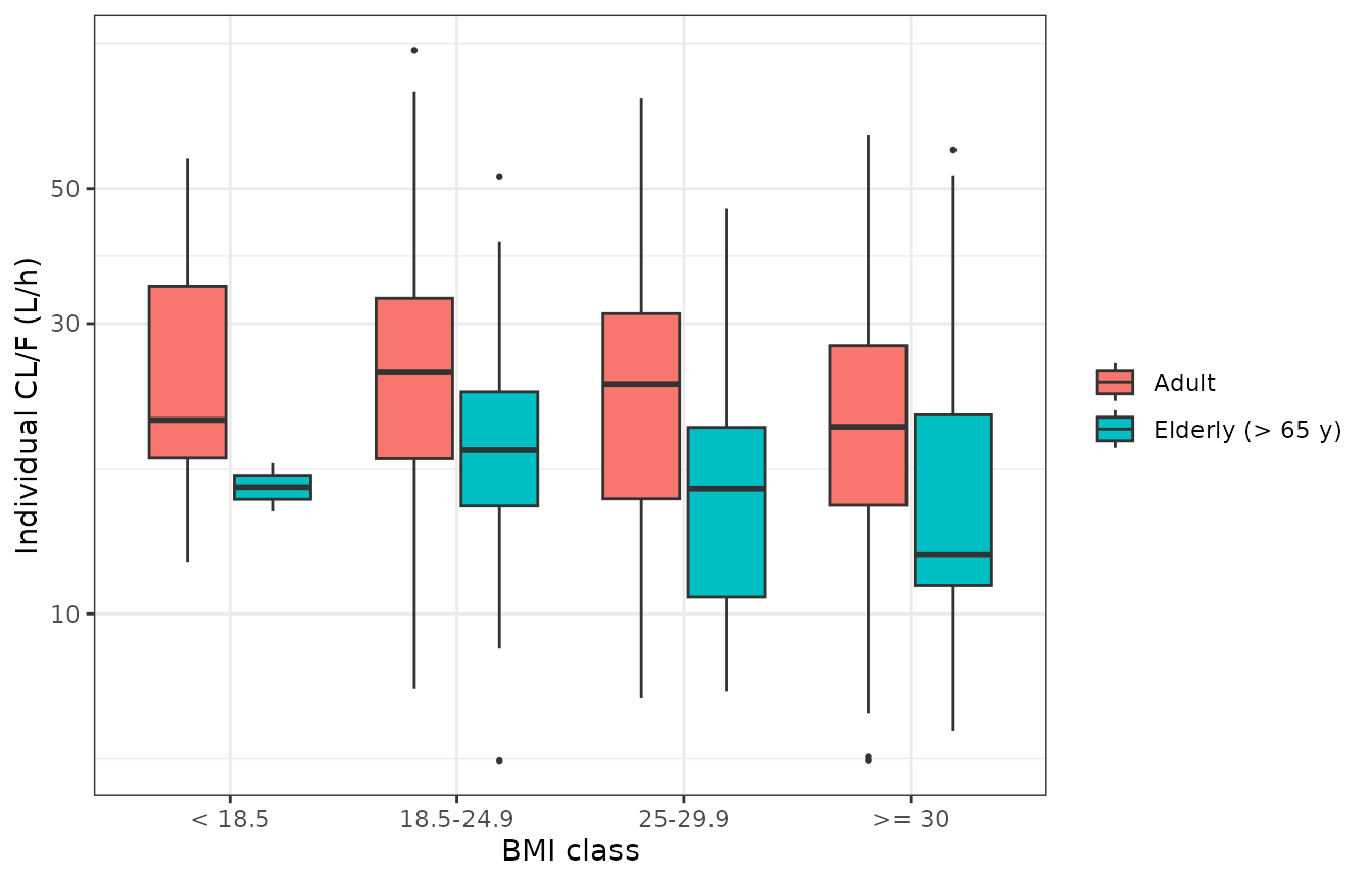

Individual CL/F by elderly status and BMI class in the virtual cohort; compare with Lalovic 2020 Figure 3.

PKNCA validation

The paper reports no NCA table, so PKNCA is used here to characterise the steady-state interval and to check the steady-state identity AUCtau = F x dose / (CL/F) subject by subject, with the individual F and CL/F from the solve.

sim_nca <- sim |>
  dplyr::filter(!is.na(Cc)) |>
  dplyr::select(id, time, Cc, treatment)

conc_obj <- PKNCA::PKNCAconc(sim_nca, Cc ~ time | treatment + id, concu = "ng/mL", timeu = "h")
dose_df <- events |>
  dplyr::filter(evid == 1) |>
  dplyr::select(id, time, amt, treatment)
dose_obj <- PKNCA::PKNCAdose(dose_df, amt ~ time | treatment + id, doseu = "mg")

intervals <- data.frame(
  start = obs_start, end = obs_start + 24,
  cmax = TRUE, tmax = TRUE, cmin = TRUE, auclast = TRUE, cav = TRUE
)
nca_res <- PKNCA::pk.nca(PKNCA::PKNCAdata(conc_obj, dose_obj, intervals = intervals))
nca_tab <- as.data.frame(nca_res)

nca_tab |>
  dplyr::filter(PPTESTCD %in% c("cmax", "tmax", "cmin", "auclast", "cav")) |>
  dplyr::group_by(treatment, PPTESTCD) |>
  dplyr::summarise(median = signif(stats::median(PPORRES), 3), .groups = "drop") |>
  tidyr::pivot_wider(names_from = PPTESTCD, values_from = median) |>
  dplyr::rename(
    Treatment = treatment, `Cmax,ss (ng/mL)` = cmax, `Tmax (h)` = tmax,
    `Cmin,ss (ng/mL)` = cmin, `AUCtau,ss (ng*h/mL)` = auclast, `Cav,ss (ng/mL)` = cav
  ) |>
  knitr::kable(caption = "Median steady-state NCA over the last 24 h interval (simulated).")

Median steady-state NCA over the last 24 h interval (simulated).

Treatment	AUCtau,ss (ng*h/mL)	Cav,ss (ng/mL)	Cmax,ss (ng/mL)	Cmin,ss (ng/mL)	Tmax (h)
10 mg	451	18.8	56.4	11.10	1
5 mg	260	10.9	29.5	7.38	1

ind <- sim |>
  dplyr::distinct(id, .keep_all = TRUE) |>
  dplyr::select(id, cl, fdepot, dose)
idchk <- nca_tab |>
  dplyr::filter(PPTESTCD == "auclast") |>
  dplyr::left_join(ind, by = "id") |>
  dplyr::mutate(ratio = PPORRES / (1000 * fdepot * dose / cl))
stopifnot(
  nrow(idchk) == 2 * n_per_arm,
  # Sparse 16-point grid: trapezoid error on the narrow peak moves the ratio a
  # few percent per subject; a transcribed CL, F or unit error moves it by tens.
  abs(stats::median(idchk$ratio) - 1) < 0.05,
  stats::quantile(abs(idchk$ratio - 1), 0.9) < 0.15
)

The individual Cav,ss is what drives the exposure-response models. Table 4 of Lalovic 2020 prints its 5th/25th/50th/75th/95th percentiles in the phase 2-3 population: 6.3/7.9/10/14/19 ng/mL at 5 mg and 12/17/21/27/37 ng/mL at 10 mg.

cav_q <- idchk |>
  dplyr::mutate(cav = PPORRES / 24) |>
  dplyr::group_by(treatment) |>
  dplyr::summarise(
    p05 = stats::quantile(cav, 0.05), p25 = stats::quantile(cav, 0.25),
    p50 = stats::median(cav), p75 = stats::quantile(cav, 0.75), p95 = stats::quantile(cav, 0.95)
  )
table4_q <- data.frame(
  treatment = c("5 mg", "10 mg"),
  t05 = c(6.3, 12), t25 = c(7.9, 17), t50 = c(10, 21), t75 = c(14, 27), t95 = c(19, 37)
)
cav_cmp <- dplyr::left_join(cav_q, table4_q, by = "treatment")
cav_cmp |>
  dplyr::mutate(dplyr::across(p05:p95, ~ signif(.x, 3))) |>
  dplyr::rename(
    Treatment = treatment, `Sim P5` = p05, `Sim P25` = p25, `Sim median` = p50,
    `Sim P75` = p75, `Sim P95` = p95, `Table 4 P5` = t05, `Table 4 P25` = t25,
    `Table 4 median` = t50, `Table 4 P75` = t75, `Table 4 P95` = t95
  ) |>
  knitr::kable(caption = "Cav,ss percentiles: virtual cohort versus Lalovic 2020 Table 4.")

Cav,ss percentiles: virtual cohort versus Lalovic 2020 Table 4.

Treatment	Sim P5	Sim P25	Sim median	Sim P75	Sim P95	Table 4 P5	Table 4 P25	Table 4 median	Table 4 P75	Table 4 P95
10 mg	5.12	11.1	18.8	34.4	84.2	12.0	17.0	21	27	37
5 mg	2.29	6.3	10.9	19.8	47.1	6.3	7.9	10	14	19

stopifnot(all(abs(cav_cmp$p50 / cav_cmp$t50 - 1) < 0.2))

The medians agree within about 10%. The simulated tails are much wider than the Table 4 ones. Table 4 was built from empirical Bayes estimates in sparsely sampled phase 3 subjects, which shrink toward the typical value, while the simulation draws the full between-subject variability, including the 68% CV on relative bioavailability.

The exposure-response models

How the coefficients were obtained

Each TEAE regression in Lalovic 2020 has the form logit(p) = intercept + slope x Cav,ss + age, sex and race terms, fitted to the pooled placebo and active data. None of the coefficients is printed. Table 4 instead prints the fitted probability for a 75-year-old White woman at ten Cav,ss values (the 5th-95th percentiles at 5 and 10 mg) and on placebo. With age, sex and race fixed at those values the logit is a straight line in Cav,ss, so the maintainers recovered the intercept and slope for that subject by least squares on qlogis(probability) against the printed Cav,ss over the ten active rows. The chunk below repeats that derivation from the transcribed table and checks that it gives the values in the model files.

table4 <- data.frame(
  cav = c(0, 6.3, 7.9, 10, 14, 19, 12, 17, 21, 27, 37),
  arm = c("Placebo", rep("5 mg", 5), rep("10 mg", 5)),
  somnolence = c(5.3, 7.2, 7.4, 7.7, 8.1, 8.9, 7.7, 8.4, 8.9, 9.6, 11.0),
  nasopharyngitis = c(8.6, 10.0, 9.5, 8.9, 8.1, 6.7, 8.9, 7.6, 6.7, 5.8, 4.0),
  uti = c(2.5, 2.0, 2.1, 2.3, 2.5, 2.9, 2.2, 2.6, 2.9, 3.3, 4.4),
  influenza = c(4.0, 3.8, 3.6, 3.4, 3.1, 2.6, 3.4, 2.9, 2.6, 2.3, 1.7),
  urti = c(3.2, 4.7, 4.4, 4.1, 3.6, 3.0, 4.1, 3.4, 3.0, 2.5, 1.7),
  headache = c(8.2, 11.0, 9.8, 9.2, 8.3, 6.8, 9.2, 7.7, 6.8, 5.7, 3.9)
)
endpoints <- c("somnolence", "nasopharyngitis", "uti", "influenza", "urti", "headache")
active <- table4$arm != "Placebo"

er_ui <- lapply(
  stats::setNames(endpoints, endpoints),
  function(ep) rxode2::rxode(readModelDb(paste0("Lalovic_2020_lemborexant_", ep)))
)

coef_chk <- dplyr::bind_rows(lapply(endpoints, function(ep) {
  y <- stats::qlogis(table4[[ep]] / 100)
  fit <- stats::lm(y[active] ~ table4$cav[active])
  th <- er_ui[[ep]]$theta
  data.frame(
    endpoint = ep,
    refit_intercept = unname(stats::coef(fit)[1]), model_intercept = th[["logit_active"]],
    refit_slope = unname(stats::coef(fit)[2]), model_slope = th[["e_cav_logit"]],
    table_placebo = y[!active], model_placebo = th[["logit_placebo"]]
  )
}))
knitr::kable(coef_chk, digits = 5, caption = "Back-solved coefficients: re-derived from Table 4 versus the values in the model files.")

Back-solved coefficients: re-derived from Table 4 versus the values in the model files.

endpoint	refit_intercept	model_intercept	refit_slope	model_slope	table_placebo	model_placebo
somnolence	-2.64443	-2.6444	0.01513	0.01513	-2.88301	-2.8830
nasopharyngitis	-1.99166	-1.9917	-0.03123	-0.03123	-2.36348	-2.3635
uti	-4.04760	-4.0476	0.02590	0.02590	-3.66356	-3.6636
influenza	-3.06895	-3.0689	-0.02646	-0.02646	-3.17805	-3.1781
urti	-2.79898	-2.7990	-0.03336	-0.03336	-3.40950	-3.4095
headache	-1.91156	-1.9116	-0.03450	-0.03450	-2.41548	-2.4155

stopifnot(
  # Same computation on both sides; the model files store 4-5 significant figures.
  all(abs(coef_chk$refit_intercept - coef_chk$model_intercept) < 5e-4),
  all(abs(coef_chk$refit_slope - coef_chk$model_slope) < 5e-5),
  all(abs(coef_chk$table_placebo - coef_chk$model_placebo) < 5e-4)
)

Reproducing Table 4

solve_er <- function(ep, cav, placebo) {
  ev <- data.frame(id = seq_along(cav), time = 0, evid = 0L, CAV = cav, PLACEBO = placebo)
  s <- rxode2::rxSolve(er_ui[[ep]], ev, returnType = "data.frame")
  100 * s[[paste0("prob_", ep)]]
}
repro <- table4[, c("cav", "arm")]
for (ep in endpoints) {
  repro[[ep]] <- solve_er(ep, table4$cav, as.integer(!active))
}
#> Warning: multi-subject simulation without without 'omega'
#> Warning: multi-subject simulation without without 'omega'
#> Warning: multi-subject simulation without without 'omega'
#> Warning: multi-subject simulation without without 'omega'
#> Warning: multi-subject simulation without without 'omega'
#> Warning: multi-subject simulation without without 'omega'
err <- as.matrix(repro[, endpoints]) - as.matrix(table4[, endpoints])

repro_show <- repro
repro_show[, endpoints] <- round(repro_show[, endpoints], 1)
repro_show |>
  dplyr::rename(
    `Cav,ss (ng/mL)` = cav, Arm = arm, Somnolence = somnolence,
    Nasopharyngitis = nasopharyngitis, `Urinary tract infection` = uti,
    Influenza = influenza, `Upper respiratory tract infection` = urti, Headache = headache
  ) |>
  knitr::kable(caption = "Replicates Table 4 of Lalovic 2020: model-predicted TEAE probability (%) for a 75-year-old White woman.")

Replicates Table 4 of Lalovic 2020: model-predicted TEAE probability (%) for a 75-year-old White woman.

Cav,ss (ng/mL)	Arm	Somnolence	Nasopharyngitis	Urinary tract infection	Influenza	Upper respiratory tract infection	Headache
0.0	Placebo	5.3	8.6	2.5	4.0	3.2	8.2
6.3	5 mg	7.2	10.1	2.0	3.8	4.7	10.6
7.9	5 mg	7.4	9.6	2.1	3.6	4.5	10.1
10.0	5 mg	7.6	9.1	2.2	3.4	4.2	9.5
14.0	5 mg	8.1	8.1	2.4	3.1	3.7	8.4
19.0	5 mg	8.7	7.0	2.8	2.7	3.1	7.1
12.0	10 mg	7.9	8.6	2.3	3.3	3.9	8.9
17.0	10 mg	8.4	7.4	2.6	2.9	3.3	7.6
21.0	10 mg	8.9	6.6	2.9	2.6	2.9	6.7
27.0	10 mg	9.7	5.5	3.4	2.2	2.4	5.5
37.0	10 mg	11.1	4.1	4.4	1.7	1.7	4.0

cat("Largest absolute difference from Table 4:", round(max(abs(err)), 2), "percentage points\n")
#> Largest absolute difference from Table 4: 0.37 percentage points
stopifnot(
  all(abs(err[!active, ]) < 0.01), # placebo row reproduced exactly
  max(abs(err[active, ])) < 0.5 # active rows within the rounding of the printed Cav,ss
)

All 66 cells are reproduced within 0.4 percentage points; the remaining difference reflects the two-significant-figure Cav,ss column. The table itself is not fully consistent at that precision: for every endpoint, the 10 mg 5th percentile (printed Cav,ss 12 ng/mL) shows the same probability as the 5 mg median (10 ng/mL), and the 10 mg median (21 ng/mL) the same as the 5 mg 95th percentile (19 ng/mL).

grid <- seq(0, 40, by = 0.5)
curves <- dplyr::bind_rows(lapply(endpoints, function(ep) {
  data.frame(endpoint = ep, cav = grid, p = solve_er(ep, grid, 0L))
}))
#> Warning: multi-subject simulation without without 'omega'
#> Warning: multi-subject simulation without without 'omega'
#> Warning: multi-subject simulation without without 'omega'
#> Warning: multi-subject simulation without without 'omega'
#> Warning: multi-subject simulation without without 'omega'
#> Warning: multi-subject simulation without without 'omega'
pts <- table4 |>
  tidyr::pivot_longer(dplyr::all_of(endpoints), names_to = "endpoint", values_to = "p") |>
  dplyr::mutate(Arm = ifelse(arm == "Placebo", "Placebo", "Lemborexant"))
ggplot2::ggplot(curves, ggplot2::aes(cav, p)) +
  ggplot2::geom_line() +
  ggplot2::geom_point(data = pts, ggplot2::aes(shape = Arm)) +
  ggplot2::facet_wrap(~endpoint, scales = "free_y") +
  ggplot2::scale_shape_manual(values = c(Lemborexant = 1, Placebo = 17)) +
  ggplot2::labs(x = "Cav,ss (ng/mL)", y = "Probability (%)", shape = NULL) +
  ggplot2::theme_bw()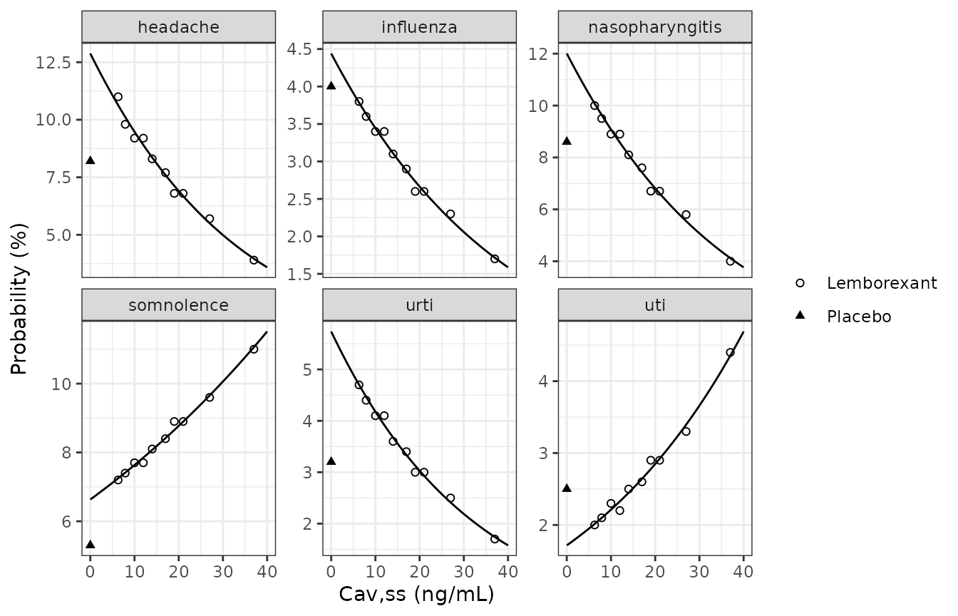

TEAE probability versus Cav,ss for a 75-year-old White woman (lines), with the Table 4 points (active: circles; placebo: triangles at Cav,ss = 0). The flat relationships are the paper’s main exposure-response finding.

Assumptions and deviations

• BMI reference value (25 kg/m^2) is not printed. Table 2 gives the BMI exponent (-0.428) and the footnote states a power form around a “generally centered reference value” without naming it. The maintainers back-solved the reference from the three BMI effect sizes in the Results (BMI 32: 11% and BMI 40: 22% higher exposure; BMI 15: 25% change in CL/F relative to “the typical subject CL/F value with a normal BMI”). 25 kg/m^2 reproduces all three; the cohort median of 26.5 kg/m^2 does not (8%, 19%, 28%), nor do 24 or 26 kg/m^2. The Table 3 ratios are independent of this choice.
• ALP reference value (71 U/L). Not printed in Table 2; 71 U/L is the Table 1 median and the value the authors assumed for the Table 3 simulations, and it reproduces the quoted ALP effect sizes.
• Elderly cut point. The Methods, the Results text and the Table 3 categories define elderly as > 65 years, which is what AGE_GT65 encodes. Table 1 and the Discussion write >= 65 years; the difference affects only subjects aged exactly 65.
• Final model versus base model. The absorption parameters and their covariate effects are fixed in the final model (Table 2) “from the base model”, but the values in Table 2 (e.g. D1 capsule 0.467 h, tablet factor 0.254, nighttime factor 2.33, Ka food factor 0.695, F1 food factor 1.21) differ from the base-model estimates in Supplemental Table S2 (0.598 h, 0.162, 1.20, 0.626, 1.28), and Table S2 has no IIV on F1 while Table 2 does. The Results text quotes the Table 2 values (0.118 h tablet D1, 2.33-fold bedtime D1, 12% higher Ka on tablet, 30% lower Ka and 21% higher F1 with food), so Table 2 is used throughout. The base-model dose >= 50 mg factor on D1 (Table S2) was dropped from the final model (Results, Final Model) and is not included.
• Sequential zero- then first-order absorption. The paper describes “mixed first-order (Ka) and zero-order (D1) absorption with a lag time” in NONMEM ADVAN12, and Supplemental Figure S2 shows a single depot-to-central arrow labelled “ka/D1”. No split fraction is reported, which identifies the usual ADVAN12 form with D1 on the depot: the dose enters the depot at a constant rate over D1 and is absorbed first-order from it. Dose records must carry rate = -2.
• Relative bioavailability. F1 is 1 in the fasted state (Table 2 reports only the food factor) and carries a fixed log-normal IIV of 68.1% CV.
• IIV and residual error scale. Table 2 reports %CV and defines CV as the square root of the variance x 100, so each variance is (CV/100)^2 and each residual proportional SD is CV/100.
• Food covariate. The Methods describe the food covariate as a standard high-fat meal, so it is carried as FED_HIGHFAT.
• Bedtime dosing is carried as DOSETIME_EVENING (the dose-record property of being taken at bedtime); the paper gives no clock-time window.
• Covariates screened but not retained. PPI use, sex, body weight and creatinine clearance are listed in covariatesDataExcluded; race, dose and the liver markers other than ALP were also screened and did not enter the final model (Results; Supplemental Figure S4).
• Exposure-response coefficients are back-solved, not printed. See the derivation above. Because Table 4 fixes age (75 years), sex (female) and race (White), the models represent that reference subject only; the source’s age, sex and race coefficients are not reported and cannot be recovered. The slope is supported only over the active Cav,ss range in Table 4 (about 6-37 ng/mL).
• Placebo in the exposure-response models. The Table 4 placebo row does not lie on the straight logit line through the active rows at Cav,ss = 0, so it is carried as its own logit, selected by PLACEBO = 1. Its six values equal the pooled incidences the Results text labels “active treatment” (for example somnolence “8.5% placebo, 5.3% active”), which suggests that the text swapped the two labels and that the Table 4 placebo row is the observed placebo proportion. The Discussion (higher somnolence on lemborexant than on placebo in both SUNRISE studies) supports that reading.
• Placeholder residual error on the probabilities. The logistic regressions have a Bernoulli likelihood with no residual term; each file carries a fixed 0.001 additive SD only so that rxode2 has an error model to attach.
• No correction notice for Lalovic 2020 was found on EuropePMC as of 2026-09-27.