Model and source
- Citation: Hirt D, Van Overmeire B, Treluyer JM, Langhendries JP, Marguglio A, Eisinger MJ, Schepens P, Urien S. An optimized ibuprofen dosing scheme for preterm neonates with patent ductus arteriosus, based on a population pharmacokinetic and pharmacodynamic study. Br J Clin Pharmacol. 2008;65(5):629-636. doi:10.1111/j.1365-2125.2008.03118.x
- Description: One-compartment population PK model with linear elimination for intravenous ibuprofen-lysine (15-min infusion) administered for closure of patent ductus arteriosus in preterm neonates (Hirt 2008). Total-body clearance increases with postnatal age via a power function (CL = 9.49 mL/h x (PNA / 96.3 h)^1.49) anchored at the cohort median PNA of 96.3 h; the apparent volume of distribution is not influenced by postnatal age, gestational age, body weight, Apgar score, or baseline serum sodium / creatinine / albumin / urine output. Exponential inter-individual variability on CL and V; proportional residual error. The PK-PD link reported by the authors (AUC1D > 600 mg L^-1 h or AUC3D > 900 mg L^-1 h associated with >= 91% PDA closure) is illustrated in the validation vignette rather than carried in this model file.
- Article: https://doi.org/10.1111/j.1365-2125.2008.03118.x
Population
Hirt 2008 studied 66 preterm neonates with haemodynamically significant patent ductus arteriosus (PDA), enrolled at Antwerp University Hospital and CHC Saint-Vincent Hospital in Liege (Belgium). Median gestational age was 28 weeks (range 25-34 weeks) and median postnatal age at the first dose was 96.3 hours (range 14-262 hours, i.e. 0.6 to 11 days). Median bodyweight at the first dose was 1015 g (range 490-1986 g). Sex distribution and race / ethnicity were not tabulated in the publication. Demographics are from Hirt 2008 Table 1.
Each neonate received three IV infusions of ibuprofen-lysine at 24 h intervals (15-min infusions via a peripheral vein with a saline flush). The intended regimen was 10 mg/kg on day 1 and 5 mg/kg on days 2 and 3, with the dose calculated from birthweight rounded to the nearest 100 g. 49 infants contributed three plasma samples, 14 contributed two, and three contributed one sample, for 129 ibuprofen concentrations total (assay LLOQ 1 mg/L, imprecision 5% CV; Hirt 2008 “Ibuprofen assay”).
The same information is available programmatically via
readModelDb("Hirt_2008_ibuprofen")$population.
Source trace
The per-parameter origin is recorded as an in-file comment next to
each ini() entry in
inst/modeldb/specificDrugs/Hirt_2008_ibuprofen.R. The table
below collects the structural equations and parameters in one place.
| Equation / parameter | Value | Source location |
|---|---|---|
One-compartment IV
(d/dt(central) = -kel * central) |
n/a | Hirt 2008 Results “Population pharmacokinetics” (ADVAN1 TRANS2) |
CL = 9.49 * (PNA / 96.3)^1.49 (mL/h with PNA in
hours) |
n/a | Hirt 2008 Results “Population pharmacokinetics” final-covariate equation |
lcl (typical CL at PNA = 96.3 h) |
log(0.00949 L/h) = log(9.49 mL/h) | Table 2 Final column: 9.49 mL/h (RSE 10%) |
lvc (typical V) |
log(0.375 L) = log(375 mL) | Table 2 Final column: 375 mL (RSE 10%) |
e_pna_cl (PNA power exponent on CL) |
1.49 | Table 2 Final column: CL, qAGE = 1.49 (RSE 17%) |
etalcl (omega^2 for log-normal IIV on CL) |
log(1 + 0.62^2) = 0.32506 | Table 2 Final column: w(CL) = 62% CV (RSE 28%) |
etalvc (omega^2 for log-normal IIV on V) |
log(1 + 0.75^2) = 0.44629 | Table 2 Final column: w(V) = 75% CV (RSE 44%) |
propSd (proportional residual SD) |
0.18 | Table 2 Final column: sigma = 18% CV (RSE 27%) |
Half-life prediction t12 = ln(2) * V / CL(PNA)
|
42.2 h at PNA 3 d, 19.7 h at 5 d, 9.8 h at 8 d | Hirt 2008 Results “Population pharmacokinetics” paragraph 4 |
| PD threshold AUC1D > 600 mg L^-1 h | 91% PDA closure | Hirt 2008 Results “Pharmacokinetic-pharmacodynamic study” + Table 3 |
Virtual cohort
The original observed data are not publicly available. The cohort below approximates the published trial demographics: PNA uniformly distributed on the observed range (14-262 h), bodyweight log-normal centred near the cohort median (1015 g, geometric SD 30% to span the observed 490-1986 g range), and the actual three-dose 10-5-5 mg/kg regimen administered as 15-min infusions on days 0, 1, and 2.
Hirt 2008 reports per-subject body weight only as the first-dose value (median 1015 g, range 490-1986 g, no day-to-day evolution table); the simulation therefore treats body weight as a per-subject constant. PNA on each subject is the value at the first dose; the model’s covariate effect uses this constant PNA on all three days (the source paper held PNA fixed at study entry for the covariate evaluation – see Methods “Patients” and Results “Population pharmacokinetics”).
set.seed(2008L)

# Helper: build one cohort as a self-contained event table. Each subject
# receives three 15-minute IV infusions of ibuprofen-lysine at 24-hour
# intervals. PNA is supplied in MONTHS (the canonical covariate column);
# the model converts back to the source-paper reference (96.3 hours)
# internally.
hours_per_month <- 30.4375 * 24    # 730.5 h / month

make_cohort <- function(n, pna_lo_h, pna_hi_h, wt_gmean_g, wt_gsd,
                        dose_day1_mg_per_kg, dose_day23_mg_per_kg,
                        label, id_offset = 0L) {
  subj <- tibble::tibble(
    id        = id_offset + seq_len(n),
    PNA_h     = runif(n, pna_lo_h, pna_hi_h),                       # hours at first dose
    WT_g      = exp(rnorm(n, log(wt_gmean_g), log(1 + wt_gsd))),    # body weight in g
    cohort    = label
  ) |>
    dplyr::mutate(
      PNA   = PNA_h / hours_per_month,                              # canonical column: months
      WT    = WT_g / 1000,                                          # canonical column: kg
      d1_mg = dose_day1_mg_per_kg  * WT,
      d23_mg = dose_day23_mg_per_kg * WT
    )

  inf_duration <- 0.25                       # 15-minute infusion
  dose_times   <- c(0, 24, 48)               # hours
  obs_times    <- sort(unique(c(
    seq(0, 72, by = 0.25),
    dose_times,
    dose_times + inf_duration
  )))

  events <- subj |>
    dplyr::rowwise() |>
    dplyr::do({
      .s <- .
      doses <- tibble::tibble(
        id   = .s$id,
        time = dose_times,
        amt  = c(.s$d1_mg, .s$d23_mg, .s$d23_mg),
        rate = c(.s$d1_mg, .s$d23_mg, .s$d23_mg) / inf_duration,
        evid = 1L,
        cmt  = "central"
      )
      obs <- tibble::tibble(
        id   = .s$id,
        time = obs_times,
        amt  = NA_real_,
        rate = NA_real_,
        evid = 0L,
        cmt  = "central"
      )
      dplyr::bind_rows(doses, obs) |>
        dplyr::arrange(time) |>
        dplyr::mutate(
          PNA    = .s$PNA,
          WT     = .s$WT,
          cohort = .s$cohort
        )
    }) |>
    dplyr::ungroup()

  list(subj = subj, events = events)
}

# Single "actual regimen" cohort spanning the full reported PNA range.
n_per_group <- 66L
built_all <- make_cohort(
  n                    = n_per_group,
  pna_lo_h             = 14,
  pna_hi_h             = 262,
  wt_gmean_g           = 1015,
  wt_gsd               = 0.30,
  dose_day1_mg_per_kg  = 10,
  dose_day23_mg_per_kg = 5,
  label                = "Actual 10-5-5 mg/kg",
  id_offset            = 0L
)

subj_all   <- built_all$subj
events_all <- built_all$events

stopifnot(!anyDuplicated(unique(events_all[, c("id", "time", "evid")])))
Simulation
mod <- readModelDb("Hirt_2008_ibuprofen")

# Stochastic simulation with full IIV and proportional residual error.
sim <- rxode2::rxSolve(
  mod,
  events = events_all,
  keep   = c("cohort", "PNA", "WT")
) |> as.data.frame()
#> ℹ parameter labels from comments will be replaced by 'label()'

# Typical-value simulation (zero random effects) for the typical-PNA
# profile and the half-life reproduction at PNA = 3 / 5 / 8 days.
mod_typ <- rxode2::zeroRe(mod)
#> ℹ parameter labels from comments will be replaced by 'label()'
Replicate published figures
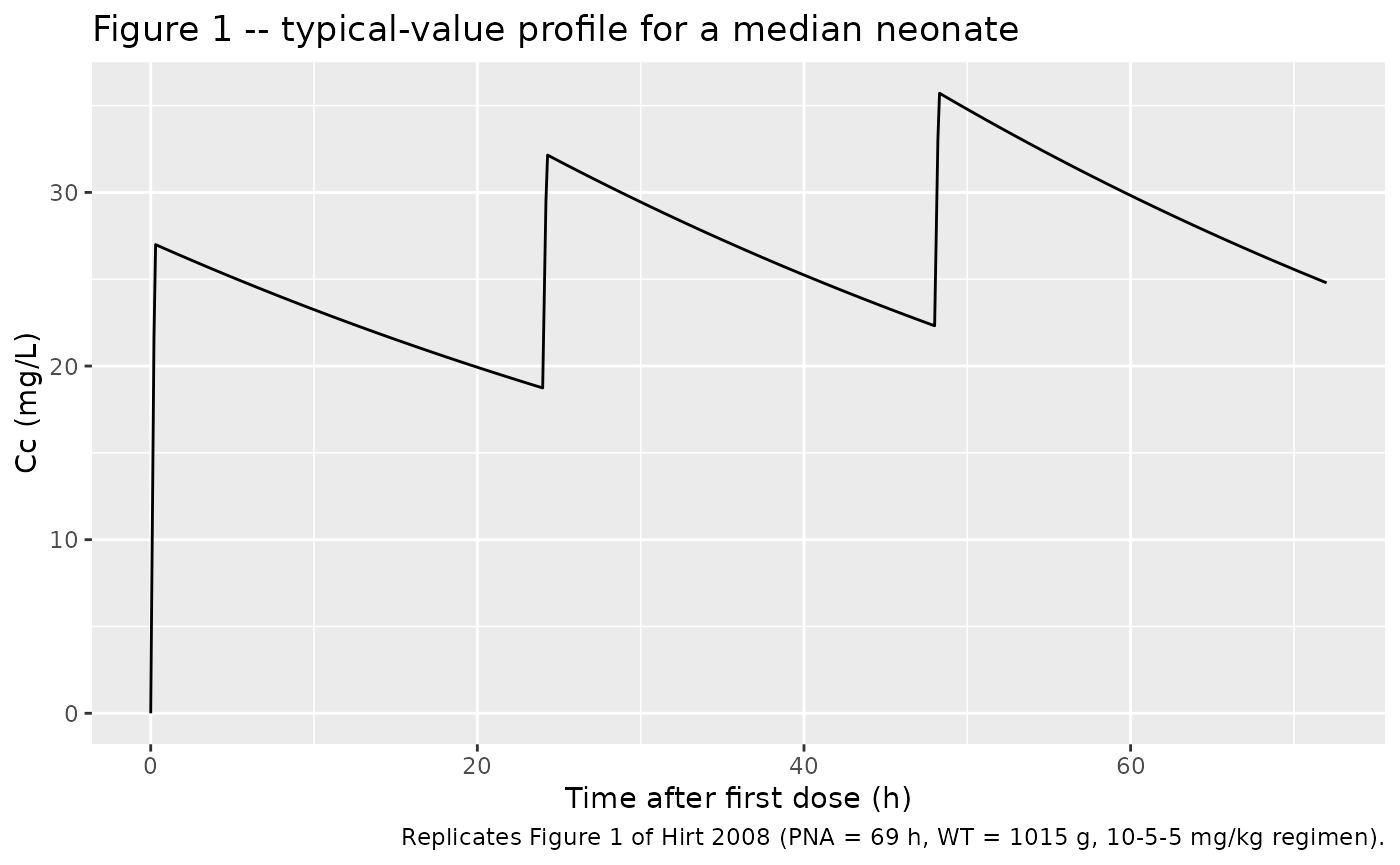
Typical concentration-time profile at the cohort-median PNA
Figure 1 of Hirt 2008 shows the population-predicted concentration-time profile for a neonate at the cohort median (PNA = 69 h, WT = 1015 g; the paper’s Figure 1 caption gives 69 h as a representative individual rather than the fitted population median of 96.3 h).
# Replicates Figure 1 of Hirt 2008: typical profile for a median neonate
# (PNA = 69 h, WT = 1015 g) receiving the 10-5-5 mg/kg regimen.
events_fig1 <- tibble::tribble(
  ~id, ~time, ~amt,             ~rate,                  ~evid, ~cmt,        ~PNA,                  ~WT,
   1L,    0,  10 * 1.015,       10 * 1.015 / 0.25,      1L,  "central",   69 / hours_per_month,  1.015,
   1L,   24,   5 * 1.015,        5 * 1.015 / 0.25,      1L,  "central",   69 / hours_per_month,  1.015,
   1L,   48,   5 * 1.015,        5 * 1.015 / 0.25,      1L,  "central",   69 / hours_per_month,  1.015
)
obs_fig1 <- tibble::tibble(
  id = 1L, time = seq(0, 72, by = 0.1),
  amt = NA_real_, rate = NA_real_, evid = 0L, cmt = "central",
  PNA = 69 / hours_per_month, WT = 1.015
)
events_fig1 <- dplyr::bind_rows(events_fig1, obs_fig1) |> dplyr::arrange(time)

sim_fig1 <- rxode2::rxSolve(mod_typ, events = events_fig1) |> as.data.frame()
#> ℹ omega/sigma items treated as zero: 'etalcl', 'etalvc'

ggplot(sim_fig1, aes(time, Cc)) +
  geom_line() +
  labs(
    x = "Time after first dose (h)",
    y = "Cc (mg/L)",
    title = "Figure 1 -- typical-value profile for a median neonate",
    caption = "Replicates Figure 1 of Hirt 2008 (PNA = 69 h, WT = 1015 g, 10-5-5 mg/kg regimen)."
  )
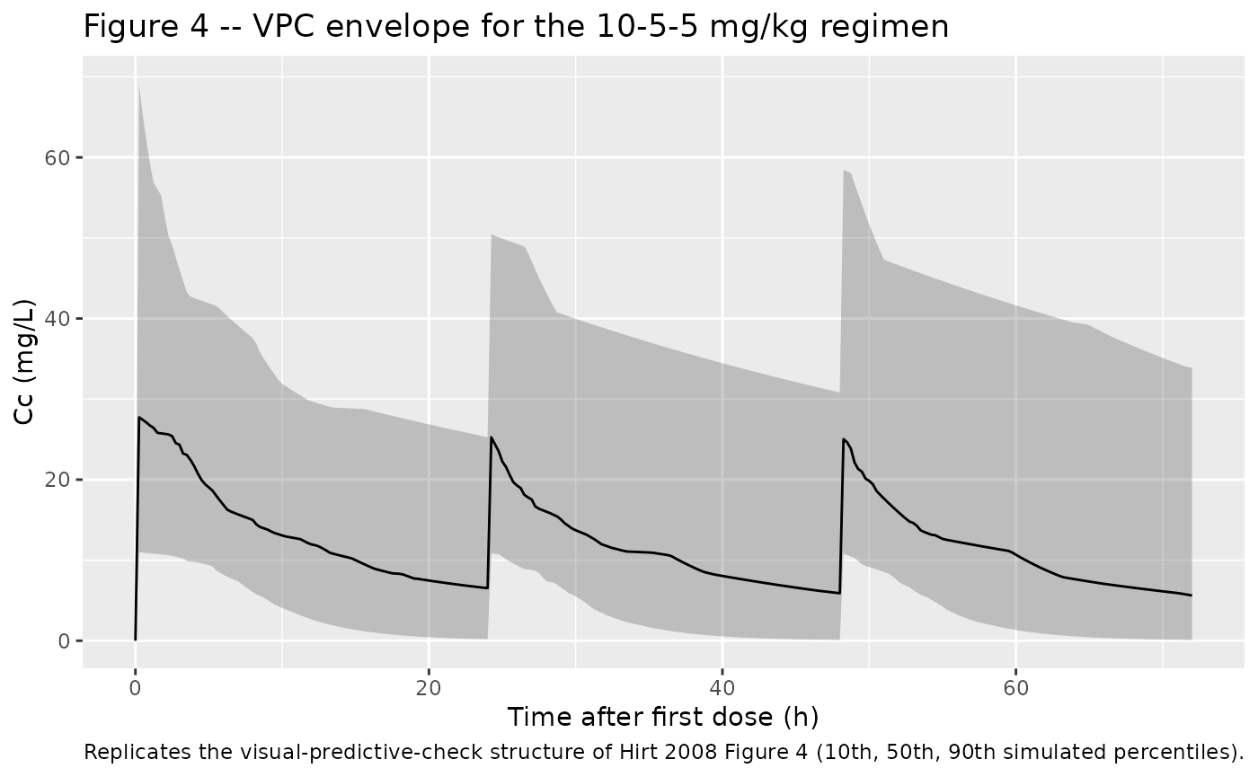
Stochastic VPC across the cohort
Figure 4 of Hirt 2008 stratifies the concentration-time courses by first-dose amount (< 10 mg, 10-15 mg, > 15 mg) and overlays the 10th / 50th / 90th percentile bands from 1000 simulations. The simulation below reproduces the cohort-wide envelope using a single first-dose amount per regimen and the proportional residual error.
# Replicates Figure 4 of Hirt 2008: VPC of Cc vs time after first dose.
vpc_bands <- sim |>
  dplyr::filter(time <= 72) |>
  dplyr::group_by(time) |>
  dplyr::summarise(
    Q10 = quantile(Cc, 0.10, na.rm = TRUE),
    Q50 = quantile(Cc, 0.50, na.rm = TRUE),
    Q90 = quantile(Cc, 0.90, na.rm = TRUE),
    .groups = "drop"
  )

ggplot(vpc_bands, aes(time, Q50)) +
  geom_ribbon(aes(ymin = Q10, ymax = Q90), alpha = 0.25) +
  geom_line() +
  labs(
    x = "Time after first dose (h)",
    y = "Cc (mg/L)",
    title = "Figure 4 -- VPC envelope for the 10-5-5 mg/kg regimen",
    caption = "Replicates the visual-predictive-check structure of Hirt 2008 Figure 4 (10th, 50th, 90th simulated percentiles)."
  )
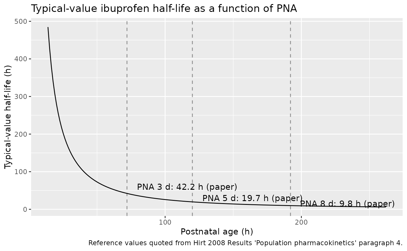
Half-life trajectory with postnatal age
The structural CL-PNA relationship implies elimination half-lives of 42.2 h at PNA = 3 days, 19.7 h at PNA = 5 days, and 9.8 h at PNA = 8 days (Hirt 2008 Results “Population pharmacokinetics” paragraph 4). The figure below traces the typical-value half-life across the studied PNA window.
pna_grid_h <- seq(14, 262, length.out = 200)
cl_typ_L_h <- 0.00949 * (pna_grid_h / 96.3) ^ 1.49
v_typ_L    <- 0.375
t12_typ_h  <- log(2) * v_typ_L / cl_typ_L_h

ggplot(data.frame(PNA_h = pna_grid_h, t12_h = t12_typ_h),
       aes(PNA_h, t12_h)) +
  geom_line() +
  geom_vline(xintercept = c(72, 120, 192), linetype = "dashed", alpha = 0.4) +
  annotate("text", x = 72,  y = 60, hjust = -0.1,
           label = "PNA 3 d: 42.2 h (paper)") +
  annotate("text", x = 120, y = 30, hjust = -0.1,
           label = "PNA 5 d: 19.7 h (paper)") +
  annotate("text", x = 192, y = 15, hjust = -0.1,
           label = "PNA 8 d: 9.8 h (paper)") +
  labs(
    x = "Postnatal age (h)",
    y = "Typical-value half-life (h)",
    title = "Typical-value ibuprofen half-life as a function of PNA",
    caption = "Reference values quoted from Hirt 2008 Results 'Population pharmacokinetics' paragraph 4."
  )
PKNCA validation
Compute AUC0-24h after the first dose (AUC1D), Cmax, Tmax, and apparent elimination half-life by PNA stratum using PKNCA. AUC1D is the pharmacodynamic-link parameter the paper uses to set the PDA-closure threshold (Hirt 2008 Table 3).
# Stratify by PNA tercile for comparison against the paper's age-band PD
# results (cohort younger than 70 h, 70-108 h, older than 108 h).
sim_with_strata <- sim |>
  dplyr::mutate(
    PNA_h     = PNA * hours_per_month,
    age_strat = dplyr::case_when(
      PNA_h <= 70  ~ "PNA <= 70 h",
      PNA_h <= 108 ~ "PNA 70-108 h",
      TRUE         ~ "PNA > 108 h"
    )
  )

pkn_in <- sim_with_strata |>
  dplyr::filter(!is.na(Cc), time <= 24) |>
  dplyr::select(id, time, Cc, treatment = age_strat)

# Defensive time-zero anchor (mandatory per pknca-recipes.md).
pkn_in <- dplyr::bind_rows(
  pkn_in,
  pkn_in |> dplyr::distinct(id, treatment) |>
    dplyr::mutate(time = 0, Cc = 0)
) |>
  dplyr::distinct(id, treatment, time, .keep_all = TRUE) |>
  dplyr::arrange(id, treatment, time)

# Dose data: only the day-1 dose enters the AUC0-24h window.
dose_pkn <- events_all |>
  dplyr::filter(evid == 1L, time == 0) |>
  dplyr::left_join(
    sim_with_strata |>
      dplyr::distinct(id, age_strat),
    by = "id"
  ) |>
  dplyr::transmute(id, time, amt, treatment = age_strat)

conc_obj <- PKNCA::PKNCAconc(pkn_in, Cc ~ time | treatment + id,
                             concu = "mg/L", timeu = "h")
dose_obj <- PKNCA::PKNCAdose(dose_pkn, amt ~ time | treatment + id,
                             doseu = "mg", route = "intravascular")

intervals <- data.frame(
  start    = 0,
  end      = 24,
  cmax     = TRUE,
  tmax     = TRUE,
  auclast  = TRUE,
  half.life = TRUE
)

nca_data <- PKNCA::PKNCAdata(conc_obj, dose_obj, intervals = intervals)
nca_res  <- PKNCA::pk.nca(nca_data)
Comparison against published half-life values
Hirt 2008 reports typical-value half-lives at three reference postnatal ages (3, 5, and 8 days). For a clean side-by-side check, simulate three typical-value cohorts at those exact PNAs and compare the PKNCA-fitted half-life against the paper’s quoted values.
typ_subj <- tibble::tribble(
  ~id, ~PNA_h, ~label,
   1L,    72L, "PNA 3 d (paper t1/2 = 42.2 h)",
   2L,   120L, "PNA 5 d (paper t1/2 = 19.7 h)",
   3L,   192L, "PNA 8 d (paper t1/2 = 9.8 h)"
)

# Typical neonate (WT = 1.015 kg); same 10-5-5 mg/kg regimen and 15-min
# infusion as the source dataset.
inf_duration <- 0.25
build_typ_events <- function(row) {
  pna_months <- row$PNA_h / hours_per_month
  doses_mg   <- 1.015 * c(10, 5, 5)
  doses <- tibble::tibble(
    id   = row$id,
    time = c(0, 24, 48),
    amt  = doses_mg,
    rate = doses_mg / inf_duration,
    evid = 1L,
    cmt  = "central",
    PNA  = pna_months,
    WT   = 1.015,
    treatment = row$label
  )
  obs <- tibble::tibble(
    id   = row$id,
    time = sort(unique(c(seq(0, 168, by = 0.5), 24, 48))),
    amt  = NA_real_,
    rate = NA_real_,
    evid = 0L,
    cmt  = "central",
    PNA  = pna_months,
    WT   = 1.015,
    treatment = row$label
  )
  dplyr::bind_rows(doses, obs) |> dplyr::arrange(time)
}

events_typ <- dplyr::bind_rows(lapply(seq_len(nrow(typ_subj)),
                                      function(i) build_typ_events(typ_subj[i, ])))

sim_typ <- rxode2::rxSolve(
  mod_typ,
  events = events_typ,
  keep   = c("treatment", "PNA", "WT")
) |> as.data.frame()
#> ℹ omega/sigma items treated as zero: 'etalcl', 'etalvc'
#> Warning: multi-subject simulation without without 'omega'

# PKNCA on the 24-72 h tail of the typical-value profile (terminal
# elimination after the third dose) for a clean t1/2 estimate.
pkn_typ_in <- sim_typ |>
  dplyr::filter(!is.na(Cc), time >= 48, time <= 168) |>
  dplyr::select(id, time, Cc, treatment)

pkn_typ_in <- dplyr::bind_rows(
  pkn_typ_in,
  pkn_typ_in |> dplyr::distinct(id, treatment) |>
    dplyr::mutate(time = 48, Cc = pkn_typ_in$Cc[match(id, pkn_typ_in$id)])
) |>
  dplyr::distinct(id, treatment, time, .keep_all = TRUE) |>
  dplyr::arrange(id, treatment, time)

# Anchor PKNCA on the time = 48 h dose event (start of the terminal
# observation window).
dose_typ <- events_typ |>
  dplyr::filter(evid == 1L, time == 48) |>
  dplyr::select(id, time, amt, treatment)

conc_typ <- PKNCA::PKNCAconc(pkn_typ_in, Cc ~ time | treatment + id,
                             concu = "mg/L", timeu = "h")
dose_typ_obj <- PKNCA::PKNCAdose(dose_typ, amt ~ time | treatment + id,
                                 doseu = "mg", route = "intravascular")

intervals_typ <- data.frame(
  start    = 48,
  end      = 168,
  half.life = TRUE
)

nca_typ_res <- PKNCA::pk.nca(PKNCA::PKNCAdata(
  conc_typ, dose_typ_obj, intervals = intervals_typ
))

reference <- tibble::tribble(
  ~treatment,                          ~half.life,
  "PNA 3 d (paper t1/2 = 42.2 h)",     42.2,
  "PNA 5 d (paper t1/2 = 19.7 h)",     19.7,
  "PNA 8 d (paper t1/2 = 9.8 h)",       9.8
)

cmp <- nlmixr2lib::ncaComparisonTable(
  simulated     = nca_typ_res,
  reference     = reference,
  by            = "treatment",
  params        = "half.life",
  units         = c(half.life = "h"),
  tolerance_pct = 10
)

knitr::kable(
  cmp,
  caption = paste(
    "Typical-value half-life by PNA stratum vs Hirt 2008 Results",
    "'Population pharmacokinetics' paragraph 4. * differs from reference",
    "by >10%."
  ),
  align = c("l", "l", "r", "r", "r")
)| NCA parameter | treatment | Reference | Simulated | % diff |
|---|---|---|---|---|
| t½ (h) | PNA 3 d (paper t1/2 = 42.2 h) | 42.2 | 42.2 | +0.1% |
| t½ (h) | PNA 5 d (paper t1/2 = 19.7 h) | 19.7 | 19.7 | +0.2% |
| t½ (h) | PNA 8 d (paper t1/2 = 9.8 h) | 9.8 | 9.8 | -0.0% |
PD link – AUC1D and PDA-closure threshold
The paper’s pharmacodynamic finding is that AUC1D > 600 mg L^-1 h is associated with 91% PDA closure (53/58 subjects), versus 50% closure when AUC1D < 600 mg L^-1 h (4/8 subjects) (Hirt 2008 Table 3). Tabulate the fraction of simulated subjects who clear the 600 mg L^-1 h threshold under the actual 10-5-5 mg/kg regimen, stratified by the PNA age bands used in the paper’s Table 4 (younger than 70 h, 70-108 h, older than 108 h).
auc1d_tbl <- as.data.frame(nca_res$result) |>
  dplyr::filter(PPTESTCD == "auclast") |>
  dplyr::select(treatment, id, AUC1D = PPORRES)

threshold_table <- auc1d_tbl |>
  dplyr::group_by(treatment) |>
  dplyr::summarise(
    n              = dplyr::n(),
    median_AUC1D   = round(median(AUC1D), 0),
    p10_AUC1D      = round(quantile(AUC1D, 0.10), 0),
    p90_AUC1D      = round(quantile(AUC1D, 0.90), 0),
    pct_above_600  = round(100 * mean(AUC1D > 600), 1),
    .groups        = "drop"
  )

threshold_table |>
  dplyr::rename(
    "PNA stratum"           = treatment,
    "Median AUC1D"          = median_AUC1D,
    "10th pct AUC1D"        = p10_AUC1D,
    "90th pct AUC1D"        = p90_AUC1D,
    "% above 600 mg L^-1 h" = pct_above_600
  ) |>
  knitr::kable(
  caption = paste(
    "Simulated AUC1D (mg L^-1 h) and percent of subjects clearing the",
    "600 mg L^-1 h threshold, stratified by PNA band. Hirt 2008 Table 4",
    "reports 91-97% PDA closure for PNA <= 70 h on the actual regimen and",
    "50% closure for PNA > 108 h, consistent with the simulated drop in",
    "AUC1D-above-threshold rate across PNA bands."
  ),
  align     = c("l", "r", "r", "r", "r", "r")
)| PNA stratum | n | Median AUC1D | 10th pct AUC1D | 90th pct AUC1D | % above 600 mg L^-1 h |
|---|---|---|---|---|---|
| PNA 70-108 h | 7 | 522 | 372 | 828 | 28.6 |
| PNA <= 70 h | 14 | 582 | 277 | 1513 | 42.9 |
| PNA > 108 h | 45 | 253 | 149 | 520 | 4.4 |
Assumptions and deviations
- Hirt 2008 reports postnatal age in hours (cohort reference 96.3 h)
but the canonical nlmixr2lib
PNAcovariate is in months. The model’smodel()block converts internally via96.3 / (30.4375 * 24)so users supply PNA in months; the source-paper formulaCL = 9.49 * (PNA / 96.3)^1.49is preserved exactly. - Body weight, gestational age, Apgar scores, baseline serum sodium /
creatinine / albumin, urine output, and occasion (day of administration)
were tested in the paper as covariates on CL and V but not retained.
They appear here under
covariatesDataExcludedto preserve the source-paper covariate screen without triggering “declared but not referenced” convention warnings. - The simulation populates the cohort by sampling PNA uniformly on the observed 14-262 h range and bodyweight from a log-normal centred near the cohort median; PNA and WT are not jointly correlated (Hirt 2008 Figure 3 and text show no significant relationship between body weight and PNA in this cohort, r^2 = 0.003, p = 0.66).
- The paper holds per-subject PNA fixed at the first-dose value for the covariate evaluation (Methods “Population pharmacokinetic modelling of ibuprofen” tested an explicit occasion / day covariate and found no significant effect on either CL or V). The simulation matches this: PNA is a per-subject constant carried on every event row.
- Sex distribution and race / ethnicity were not tabulated in Hirt
2008, so
sex_female_pctisNAandrace_ethnicityisNULLin the modelpopulationmetadata. - The PD endpoint (PDA closure rate as a function of AUC1D and AUC3D) is illustrated downstream in the vignette via the AUC-threshold table rather than carried in the model file; ibuprofen’s effect on PDA closure is a logistic-regression observation, not a structural PK / PD model in the source paper.
- The half-life comparison in the PKNCA section computes PKNCA’s terminal half-life on the 48-168 h tail of a typical-value, no-IIV simulation, so the estimate reflects the structural CL / V relationship without contributions from inter-individual variability or residual error. The paper’s quoted values (42.2, 19.7, 9.8 h) are likewise typical-value half-lives derived from the same structural equations.