Tenofovir and emtricitabine mucosal tissue PK (Leung 2023)
Source:vignettes/articles/Leung_2023_tenofovir_emtricitabine.Rmd
Leung_2023_tenofovir_emtricitabine.RmdModel and source
Leung et al. (2023) fitted the same 16-compartment semi-physiological model separately to tenofovir (TFV, given as tenofovir disoproxil fumarate, TDF) and to emtricitabine (FTC). The package therefore carries two models that share one structure and one article:
-
Leung_2023_tenofovir: Semi-physiological 16-compartment population PK model for tenofovir (TFV) after a single oral dose of tenofovir disoproxil fumarate (TDF) in healthy premenopausal women (Leung 2023). The oral depot feeds a two-compartment plasma model by first-order absorption (ka) and, in parallel, a seven-stage gut-transit chain (ktr) whose last stage delivers drug to rectal tissue (ka_rectum) or out of the body (kel_gut). The total plasma clearance CLtt is routed as fixed fractions into vaginal, cervical and rectal tissue (fcl_); each tissue holds parent TFV, cleared at cl_ , of which the fraction fm_ forms the active intracellular metabolite tenofovir diphosphate (TFV-DP) in a separate tissue state cleared at cl_ _tfvdp. Tissue volumes are fixed to physiological tissue weights (density 1 g/mL). Amounts in nmol, concentrations in nmol/L; dose the TFV molar equivalent of the TDF dose (mg TDF / 635.52 x 1e6 nmol) into depot. Seven outputs: plasma TFV and TFV / TFV-DP in each of the three tissues. -
Leung_2023_emtricitabine: Semi-physiological 16-compartment population PK model for emtricitabine (FTC) after a single oral dose in healthy premenopausal women (Leung 2023). The oral depot feeds a two-compartment plasma model by first-order absorption (ka) and, in parallel, a seven-stage gut-transit chain (ktr) whose last stage delivers drug to rectal tissue (ka_rectum) or out of the body (kel_gut). The total plasma clearance CLtt is routed as fixed fractions into vaginal, cervical and rectal tissue (fcl_); each tissue holds parent FTC, cleared at cl_ , of which the fraction fm_ forms the active intracellular metabolite emtricitabine triphosphate (FTC-TP) in a separate tissue state cleared at cl_ _ftctp. Tissue volumes are fixed to physiological tissue weights (density 1 g/mL). Amounts in nmol, concentrations in nmol/L; dose the FTC dose in nmol (mg / 247.24 x 1e6) into depot. Seven outputs: plasma FTC and FTC / FTC-TP in each of the three tissues. - Citation: Leung E, Cottrell ML, Sykes C, White N, Kashuba ADM, Dumond JB. A multicompartment population PK model to predict tenofovir and emtricitabine mucosal tissue concentrations for HIV prevention. CPT Pharmacometrics Syst Pharmacol. 2023;12(12):1922. doi:10.1002/psp4.13042
- Article: https://doi.org/10.1002/psp4.13042 (open access, PMC10725258)
- Supplement: Appendix S1 (Tables S1-S2, Figures S1-S7) and Appendix
S2 (the two final NONMEM 7.3 control streams,
run15for FTC andrun17for TFV).
Population
The data came from a phase I, open-label, single-dose study in healthy, premenopausal, HIV-negative women (NCT01330199, University of North Carolina). Participants took one oral dose of TDF 150, 300 or 600 mg or of FTC 100, 200 or 400 mg. Plasma was sampled intensively over 48 h. Each participant gave one vaginal, one cervical and one rectal biopsy at 6, 12, 24 or 48 h post-dose.
Twenty-three participants were modelled for each drug. The TFV dataset had 413 observations: 275 in plasma plus 23 TFV and 23 TFV-DP in each tissue. The FTC dataset had 573. Supplementary Table S1 gives the demographics of the enrolled arms. The TDF arm (N = 25) had median age 27 years, weight 67.4 kg and BMI 24.1 kg/m^2, and was 64% Caucasian, 32% African American and 4% Asian American. The FTC arm (N = 24) had median age 22 years, weight 62.8 kg and BMI 22.5 kg/m^2, and was 75% Caucasian, 16.7% African American, 4.2% Asian American and 4.2% American Indian. The paper tested no covariates because the population was homogeneous.
str(readModelDb("Leung_2023_tenofovir")()$population)
#> List of 14
#>  $ species       : chr "human"
#>  $ n_subjects    : int 23
#>  $ n_studies     : int 1
#>  $ age_range     : chr "IQR 22.75-31.25 years (TDF arm, N = 25 enrolled)"
#>  $ age_median    : chr "27 years"
#>  $ weight_range  : chr "IQR 60.4-76.8 kg"
#>  $ weight_median : chr "67.4 kg"
#>  $ bmi_median    : chr "24.1 kg/m^2 (IQR 21.6-26.9)"
#>  $ sex_female_pct: num 100
#>  $ race_ethnicity: Named num [1:3] 64 32 4
#>   ..- attr(*, "names")= chr [1:3] "White" "Black" "Asian"
#>  $ disease_state : chr "Healthy premenopausal HIV-negative women (phase I dose-ranging tissue PK study, NCT01330199)"
#>  $ dose_range    : chr "Single oral dose of TDF 150, 300 or 600 mg (7, 8 and 8 modelled participants)"
#>  $ regions       : chr "USA (University of North Carolina)"
#>  $ notes         : chr "Demographics from Leung 2023 Table S1 (25 enrolled in the TDF arm); 23 participants with 413 observations were "| __truncated__
Model structure
Figure 1 of the paper and both control streams give the same structure:
- The oral dose sits in
depot. It empties in parallel into plasma (central, rateka) and into a seven-stage gut-transit chain (transit1totransit7, ratektr= Kg). The depot therefore loseska + ktr, and only the fractionka / (ka + ktr)of the dose reaches plasma. - Plasma is a two-compartment model (
central,peripheral1). - The total plasma clearance
cl(CLtt) leaves plasma in full. The fractionsfcl_vagina,fcl_cervixandfcl_rectum(Fv, Fe, Fr) of it carry drug into the three tissues, and the remainder1 - Fv - Fe - Fris eliminated (Equation 1). - Each tissue holds the parent drug (
vagina,cervix,rectum), cleared atcl_<tissue>(CLttvvtp, CLttve, CLttvr). The fractionfm_<tissue>(Fvt, Fet, Frt) of that loss forms the phosphorylated anabolite in the same tissue (<tissue>_tfvdpor<tissue>_ftctp), which is cleared atcl_<tissue>_<metab>(CLvvtp, CLvetp, CLvrtp). The rest is lost in mucosal secretions (Equations 2-3). - The last gut-transit stage moves drug into rectal tissue
(
ka_rectum, Kga) and out of the body (kel_gut, Kgr). This produces the delayed second rise of the rectal concentrations. - The tissue volumes are fixed to physiological tissue weights at a density of 1 g/mL: vagina 0.09 L, cervix 0.01 L, rectum 0.17 L. The same volume is used for the parent and the metabolite state.
Amounts are in nmol and concentrations in nmol/L. A TDF dose in mg
becomes mg / 635.52 * 1e6 nmol of TFV (one TFV per TDF, MW
635.52 g/mol). An FTC dose becomes mg / 247.24 * 1e6
nmol.
Source trace
Every ini() value carries an in-file comment pointing to
its source. The table collects them. “CS” is the control stream in
Appendix S2.
| Parameter (model name) | TFV | FTC | Source |
|---|---|---|---|
Ka (lka), 1/h |
0.863 | 0.649 | Table 1 |
Vc (lvc), L |
331 | 72.3 | Table 1 |
Vp (lvp), L |
843 | 122 | Table 1 |
Q (lq), L/h |
142 | 6.06 | Table 1 |
CLtt (lcl), L/h |
58.7 | 18.9 | Table 1 |
Fv (lfcl_vagina) |
7.90e-5 | 1.31e-3 | Table 1 (x 1e-5 column) |
Fe (lfcl_cervix) |
1.50e-5 | 6.90e-5 | Table 1 |
Fr (lfcl_rectum) |
7.00e-5, fixed | 4.01e-3 | Table 1; TFV CS THETA(8) 0.00007 FIX
|
Fvt (fm_vagina) |
0.243 | 0.325 | Table 1 |
CLttvvtp (lcl_vagina), L/h |
0.0111 | 0.0101 | Table 1 (FTC printed 0101; see Assumptions) |
CLvvtp (lcl_vagina_<metab>), L/h |
0.0410 | 0.0399 | Table 1 |
Fet (fm_cervix) |
0.0292 | 1, fixed | Table 1, footnote a; FTC CS THETA(14) |
CLttve (lcl_cervix), L/h |
1.83e-3 | 0.947e-3 | Table 1 (x 1e-3 column) |
CLvetp (lcl_cervix_<metab>), L/h |
2.07e-3 | 8.2e-3 | Table 1 (x 1e-3 column) |
Frt (fm_rectum) |
1, fixed | 0.0107 | Table 1, footnote a; TFV CS THETA(19) |
CLttvr (lcl_rectum), L/h |
4.77e-3 | 22.3e-3 | Table 1 (x 1e-3 column) |
CLvrtp (lcl_rectum_<metab>), L/h |
0.140 | 0.647 | Table 1 |
Vv, Vvtp / Ve, Vetp / Vr, Vrtp (lv_*), L |
0.09 / 0.01 / 0.17, fixed | same | Methods, Results; CS THETA(11)-(12), (16)-(17), (21)-(22) |
Kg (lktr), 1/h |
0.0752 | 0.0724 | Table 1 |
Kga (lka_rectum), 1/h |
0.0589 | 1, fixed | Table 1, footnote a |
Kgr (lkel_gut), 1/h |
1, fixed | 1, fixed | Table 1, footnote a |
| IIV Ka / Vc, %CV | 37.7 / 39.0 | 51.7 / 20.5 | Table 1 |
| IIV CLtt, %CV (corr. with Vc) | 22.7 (100%) | none | Table 1; TFV CS $OMEGA BLOCK(2)
|
| IIV CLttvvtp / CLttve / CLttvr, %CV | none | 38.3 / 34.4 / 87 | Table 1; FTC CS ETA(3), ETA(5), ETA(7) |
| IIV CLvvtp / CLvetp, %CV | 97.6 / 172 | 39.9 / 164.9 | Table 1 |
| IIV Kg, %CV | 87.8 | 70.1 | Table 1 |
| Proportional RUV, plasma / vagina / vagina metab., %CV | 28.4 / 39.1 / 42.3 | 31.6 / 24.2 / 83.1 | Table 1 |
| Proportional RUV, cervix / cervix metab., %CV | 42.0 / 31.1 | 66.9 / 58.2 | Table 1 |
| Proportional RUV, rectum / rectum metab., %CV | 51.3 / 56.5 | 1.51 / 81.9 | Table 1 (rectal metabolite row printed as ‘Metabolite in plasma’) |
Depot outflow -(ka + ktr) * depot
|
CS K1T2 = Ka, K1T10 = Kg
|
||
| Plasma and tissue ODEs | Equations 1-3; Figure 1; CS $PK
|
Virtual cohort and simulation
The cohort reproduces the study design: three dose arms per drug
(50%, 100% and 200% of the licensed dose), 100 virtual participants per
arm, one dose at time 0, and observations to 48 h. Both models declare
seven endpoints, so the observation rows name the plasma state
(cmt = "central") and set dvid = 1; rxode2
then returns every concentration column on every row.
set.seed(20231201)
rxode2::rxSetSeed(20231201)

obs_times <- c(0, 0.25, 0.5, 1, 1.5, 2, 3, 4, 6, 8, 10, 12, 16, 20, 24, 30, 36, 42, 48)
mw <- c(TFV = 635.52, FTC = 247.24)
n_per_arm <- 100L

make_arm <- function(drug, dose_mg, id_offset) {
  ids <- id_offset + seq_len(n_per_arm)
  amt <- dose_mg / mw[[drug]] * 1e6
  dose <- data.frame(
    id = ids, time = 0, amt = amt, evid = 1L, cmt = "depot",
    dvid = NA_integer_
  )
  obs <- expand.grid(id = ids, time = obs_times) |>
    mutate(amt = 0, evid = 0L, cmt = "central", dvid = 1L)
  bind_rows(dose, obs) |>
    mutate(drug = drug, dose_mg = dose_mg, dose_nmol = amt[1]) |>
    arrange(id, time, desc(evid))
}

arms <- data.frame(
  drug = c("TFV", "TFV", "TFV", "FTC", "FTC", "FTC"),
  dose_mg = c(150, 300, 600, 100, 200, 400),
  ref_mg = c(300, 300, 300, 200, 200, 200)
)
events <- bind_rows(lapply(seq_len(nrow(arms)), function(i) {
  make_arm(arms$drug[i], arms$dose_mg[i], (i - 1L) * n_per_arm)
})) |>
  mutate(arm = paste(drug, dose_mg, "mg"))
stopifnot(!anyDuplicated(events[events$evid == 1, "id"]))
mod_tfv <- readModelDb("Leung_2023_tenofovir")
mod_ftc <- readModelDb("Leung_2023_emtricitabine")

conc_cols <- function(sim, metab) {
  sim |>
    as.data.frame() |>
    rename_with(~ sub(paste0("_", metab, "$"), "_metab", .x))
}

sim_tfv <- rxSolve(mod_tfv, events = filter(events, drug == "TFV"),
                   keep = c("drug", "arm", "dose_mg", "dose_nmol")) |>
  conc_cols("tfvdp")
#> ℹ parameter labels from comments will be replaced by 'label()'
sim_ftc <- rxSolve(mod_ftc, events = filter(events, drug == "FTC"),
                   keep = c("drug", "arm", "dose_mg", "dose_nmol")) |>
  conc_cols("ftctp")
#> ℹ parameter labels from comments will be replaced by 'label()'

out_cols <- c("Cc", "Cvagina", "Cvagina_metab", "Ccervix", "Ccervix_metab",
              "Crectum", "Crectum_metab")
sim <- bind_rows(sim_tfv, sim_ftc) |>
  select(id, time, drug, arm, dose_mg, dose_nmol, all_of(out_cols)) |>
  left_join(arms, by = c("drug", "dose_mg"))
Replicate published figures
The model is linear, so the pcVPCs of Figure 3 (and Figures S5-S6),
which pool the three arms after normalising them to the licensed dose,
correspond to dose-normalised simulated concentrations
(C * ref_mg / dose_mg). The bands below are the 5th, 50th
and 95th percentiles of the individual predictions; residual error is
not added.
matrix_labels <- c(
  Cc = "Plasma, parent", Cvagina = "Vaginal tissue, parent",
  Cvagina_metab = "Vaginal tissue, metabolite", Ccervix = "Cervical tissue, parent",
  Ccervix_metab = "Cervical tissue, metabolite", Crectum = "Rectal tissue, parent",
  Crectum_metab = "Rectal tissue, metabolite"
)
# Pre-dose concentrations are zero and cannot be drawn on a log axis.
sim_post <- sim[sim$time > 0, ]
vpc <- sim_post |>
  pivot_longer(all_of(out_cols), names_to = "output", values_to = "conc") |>
  mutate(conc_norm = conc * ref_mg / dose_mg) |>
  group_by(drug, output, time) |>
  summarise(
    Q05 = quantile(conc_norm, 0.05), Q50 = median(conc_norm),
    Q95 = quantile(conc_norm, 0.95), .groups = "drop"
  ) |>
  mutate(
    output = factor(matrix_labels[output], levels = matrix_labels),
    drug = factor(drug, levels = c("TFV", "FTC"))
  )

ggplot(vpc, aes(time, Q50)) +
  geom_ribbon(aes(ymin = Q05, ymax = Q95), fill = "steelblue", alpha = 0.3) +
  geom_line(colour = "firebrick") +
  facet_grid(output ~ drug, scales = "free_y") +
  scale_y_log10() +
  scale_x_continuous(breaks = seq(0, 48, 12)) +
  labs(
    x = "Time after dose (h)",
    y = "Dose-normalised concentration (nmol/L)",
    title = "Simulated 5th-50th-95th percentiles, normalised to TDF 300 mg / FTC 200 mg",
    caption = "Replicates Figure 3 (plasma, vaginal and rectal parent) and Figures S5-S6 (cervix, metabolites) of Leung 2023."
  ) +
  theme(strip.text.y = element_text(size = 7))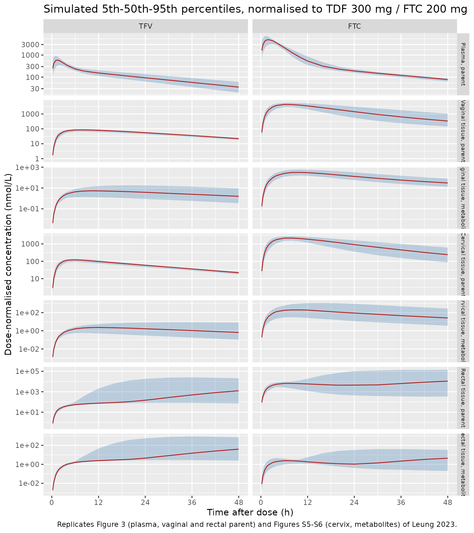
Typical values against Figure 3
The table below compares the typical-value profile (random effects set to zero) with the median of the simulated band in Figure 3, read off the log-scaled panels by eye. Those readings are approximate, to roughly a factor of 1.5, so the check catches gross errors such as a wrong dose unit, a misplaced power of ten or a wrong fraction. It cannot detect a 10% difference.
typ_events <- bind_rows(
  make_arm("TFV", 300, 0) |> filter(id == 1),
  make_arm("FTC", 200, 0) |> filter(id == 1)
)
typ <- bind_rows(
  rxSolve(zeroRe(mod_tfv), filter(typ_events, drug == "TFV"), keep = "drug") |>
    conc_cols("tfvdp"),
  rxSolve(zeroRe(mod_ftc), filter(typ_events, drug == "FTC"), keep = "drug") |>
    conc_cols("ftctp")
)
#> ℹ parameter labels from comments will be replaced by 'label()'
#> ℹ omega/sigma items treated as zero: 'etalka', 'etalvc', 'etalcl', 'etalcl_vagina_tfvdp', 'etalcl_cervix_tfvdp', 'etalktr'
#> ℹ parameter labels from comments will be replaced by 'label()'
#> ℹ omega/sigma items treated as zero: 'etalka', 'etalvc', 'etalcl_vagina', 'etalcl_vagina_ftctp', 'etalcl_cervix', 'etalcl_cervix_ftctp', 'etalcl_rectum', 'etalktr'

# Approximate medians read from Figure 3 (nmol/L, licensed-dose normalised).
fig3 <- tribble(
  ~drug, ~output, ~time, ~figure,
  "TFV", "Cc", 1.5, 600,
  "TFV", "Cc", 48, 35,
  "TFV", "Cvagina", 6, 85,
  "TFV", "Cvagina", 24, 50,
  "TFV", "Cvagina", 48, 20,
  "TFV", "Crectum", 6, 60,
  "TFV", "Crectum", 24, 160,
  "TFV", "Crectum", 48, 1500,
  "FTC", "Cc", 2, 5000,
  "FTC", "Cc", 48, 80,
  "FTC", "Cvagina", 6, 4500,
  "FTC", "Cvagina", 24, 1300,
  "FTC", "Cvagina", 48, 350,
  "FTC", "Crectum", 6, 6000,
  "FTC", "Crectum", 24, 5000,
  "FTC", "Crectum", 48, 9500
)
typ_cmp <- typ |>
  select(drug, time, all_of(out_cols)) |>
  pivot_longer(all_of(out_cols), names_to = "output", values_to = "model") |>
  inner_join(fig3, by = c("drug", "output", "time")) |>
  mutate(ratio = model / figure)

typ_cmp |>
  mutate(output = matrix_labels[output], model = signif(model, 3), ratio = round(ratio, 2)) |>
  rename(
    Drug = drug, Output = output, "Time (h)" = time,
    "Model typical value (nmol/L)" = model, "Figure 3 median, approx. (nmol/L)" = figure,
    "Model / figure" = ratio
  ) |>
knitr::kable()| Drug | Time (h) | Output | Model typical value (nmol/L) | Figure 3 median, approx. (nmol/L) | Model / figure |
|---|---|---|---|---|---|
| TFV | 1.5 | Plasma, parent | 607.0 | 600 | 1.01 |
| TFV | 6.0 | Vaginal tissue, parent | 86.3 | 85 | 1.02 |
| TFV | 6.0 | Rectal tissue, parent | 54.5 | 60 | 0.91 |
| TFV | 24.0 | Vaginal tissue, parent | 55.7 | 50 | 1.11 |
| TFV | 24.0 | Rectal tissue, parent | 161.0 | 160 | 1.01 |
| TFV | 48.0 | Plasma, parent | 35.8 | 35 | 1.02 |
| TFV | 48.0 | Vaginal tissue, parent | 22.2 | 20 | 1.11 |
| TFV | 48.0 | Rectal tissue, parent | 1380.0 | 1500 | 0.92 |
| FTC | 2.0 | Plasma, parent | 5140.0 | 5000 | 1.03 |
| FTC | 6.0 | Vaginal tissue, parent | 4500.0 | 4500 | 1.00 |
| FTC | 6.0 | Rectal tissue, parent | 6920.0 | 6000 | 1.15 |
| FTC | 24.0 | Vaginal tissue, parent | 1410.0 | 1300 | 1.08 |
| FTC | 24.0 | Rectal tissue, parent | 2720.0 | 5000 | 0.54 |
| FTC | 48.0 | Plasma, parent | 77.9 | 80 | 0.97 |
| FTC | 48.0 | Vaginal tissue, parent | 332.0 | 350 | 0.95 |
| FTC | 48.0 | Rectal tissue, parent | 12000.0 | 9500 | 1.27 |
# Every point is within a factor of 2 of the figure. The ratios are not tight,
# because the figure readings are approximate, but a dose-unit or power-of-ten
# error would move them by 10-fold or more.
stopifnot(all(typ_cmp$ratio > 0.5 & typ_cmp$ratio < 2))
The lowest ratio is FTC in rectal tissue at 24 h, at about 0.54. The typical rectal FTC profile falls to a trough near 24 h and then climbs again as the gut-transit chain delivers unabsorbed drug (36 h: about 5700 nmol/L; 48 h: about 12000 nmol/L). The figure’s band for that time spans the 18-36 h bin, so it averages over the trough and the start of the climb, and it sits above the 24 h trough value. The observed median line in the same panel dips to about 2500 nmol/L at 24 h, close to the model’s typical value.
Mass balance of the absorbed fraction
The depot empties into plasma and into the gut-transit chain in
parallel. So the plasma exposure of a typical subject is
AUC = dose * ka / (ka + ktr) / CLtt, and the rest of the
dose goes down the gut. The simulated plasma AUC (trapezoids on a fine
grid to 2000 h) must match this closed form. Both sides use the same
typical parameters, so the tolerance is tight.
fine <- c(seq(0, 48, by = 0.05), seq(48.5, 2000, by = 0.5))

auc_mass_balance <- function(mod, dose_nmol) {
  m <- mod()
  ka <- exp(m$theta[["lka"]])
  ktr <- exp(m$theta[["lktr"]])
  ev <- data.frame(
    id = 1L, time = c(0, fine), amt = c(dose_nmol, rep(0, length(fine))),
    evid = c(1L, rep(0L, length(fine))),
    cmt = c("depot", rep("central", length(fine))),
    dvid = c(NA_integer_, rep(1L, length(fine)))
  )
  s <- as.data.frame(rxSolve(zeroRe(m), ev))
  c(
    simulated = sum(diff(s$time) * (head(s$Cc, -1) + tail(s$Cc, -1)) / 2),
    closed_form = dose_nmol * ka / (ka + ktr) / exp(m$theta[["lcl"]]),
    fraction_to_plasma = ka / (ka + ktr)
  )
}
auc_tab <- as.data.frame(rbind(
  TFV = auc_mass_balance(mod_tfv, 300 / mw[["TFV"]] * 1e6),
  FTC = auc_mass_balance(mod_ftc, 200 / mw[["FTC"]] * 1e6)
))
#> ℹ omega/sigma items treated as zero: 'etalka', 'etalvc', 'etalcl', 'etalcl_vagina_tfvdp', 'etalcl_cervix_tfvdp', 'etalktr'
#> ℹ omega/sigma items treated as zero: 'etalka', 'etalvc', 'etalcl_vagina', 'etalcl_vagina_ftctp', 'etalcl_cervix', 'etalcl_cervix_ftctp', 'etalcl_rectum', 'etalktr'
knitr::kable(signif(auc_tab, 4), caption = "Typical plasma AUC0-inf (nmol*h/L) and fraction of the dose absorbed into plasma.")| simulated | closed_form | fraction_to_plasma | |
|---|---|---|---|
| TFV | 7397 | 7397 | 0.9198 |
| FTC | 38500 | 38510 | 0.8996 |
PKNCA validation
Plasma NCA per drug and dose arm. The paper reports no NCA values, so there is no published table to compare against. The check is that exposure is dose-proportional (the model is linear) and that the median AUC matches the closed form above.
sim_nca <- sim |>
  filter(!is.na(Cc)) |>
  select(id, time, Cc, arm)
sim_nca <- bind_rows(
  sim_nca,
  sim_nca |> distinct(id, arm) |> mutate(time = 0, Cc = 0)
) |>
  distinct(id, arm, time, .keep_all = TRUE) |>
  arrange(id, arm, time)

dose_df <- events |>
  filter(evid == 1) |>
  select(id, time, amt, arm)

conc_obj <- PKNCA::PKNCAconc(sim_nca, Cc ~ time | arm + id)
dose_obj <- PKNCA::PKNCAdose(dose_df, amt ~ time | arm + id)
intervals <- data.frame(
  start = 0, end = Inf,
  cmax = TRUE, tmax = TRUE, aucinf.obs = TRUE, half.life = TRUE
)
nca_res <- PKNCA::pk.nca(PKNCA::PKNCAdata(conc_obj, dose_obj, intervals = intervals))

nca_summary <- as.data.frame(nca_res) |>
  filter(PPTESTCD %in% c("cmax", "tmax", "aucinf.obs", "half.life")) |>
  group_by(arm, PPTESTCD) |>
  summarise(median = median(PPORRES, na.rm = TRUE), .groups = "drop") |>
  pivot_wider(names_from = PPTESTCD, values_from = median) |>
  left_join(distinct(events, arm, drug, dose_mg), by = "arm") |>
  arrange(desc(drug), dose_mg) |>
  mutate(auc_per_mg = aucinf.obs / dose_mg)

nca_summary |>
  mutate(across(c(cmax, aucinf.obs, half.life, auc_per_mg), ~ signif(.x, 3))) |>
  select(arm, cmax, tmax, aucinf.obs, half.life, auc_per_mg) |>
  rename(
    Arm = arm, "Cmax (nmol/L)" = cmax, "Tmax (h)" = tmax,
    "AUC0-inf (nmol*h/L)" = aucinf.obs, "Half-life (h)" = half.life,
    "AUC0-inf per mg" = auc_per_mg
  ) |>
knitr::kable(caption = "Median simulated plasma NCA by arm (100 participants per arm).")| Arm | Cmax (nmol/L) | Tmax (h) | AUC0-inf (nmol*h/L) | Half-life (h) | AUC0-inf per mg |
|---|---|---|---|---|---|
| TFV 150 mg | 284 | 1.5 | 3530 | 16.9 | 23.5 |
| TFV 300 mg | 607 | 1.5 | 7370 | 17.2 | 24.6 |
| TFV 600 mg | 1270 | 1.5 | 14900 | 17.2 | 24.9 |
| FTC 100 mg | 2450 | 2.0 | 18900 | 19.0 | 189.0 |
| FTC 200 mg | 5080 | 2.0 | 38200 | 19.1 | 191.0 |
| FTC 400 mg | 10500 | 2.0 | 76900 | 19.0 | 192.0 |
# Dose proportionality: within each drug the AUC per mg differs between arms
# only by sampling noise, because the model is linear.
prop_check <- nca_summary |>
  group_by(drug) |>
  summarise(spread = max(auc_per_mg) / min(auc_per_mg))
stopifnot(all(prop_check$spread < 1.3))

# The terminal half-life over 48 h reflects the distribution phase, so it is
# reported, not asserted.
Assumptions and deviations
-
FTC CLttvvtp. Table 1 prints the FTC value as
0101, with the decimal point lost. The maintainers read it as 0.0101 L/h. The control-stream initial estimate is 0.0123 with an upper bound of 1, which rules out 1.01, and 0.101 fails against Figure 3e. With 0.0101 the typical vaginal FTC concentration is about 4500 nmol/L at 6 h and 1400 nmol/L at 24 h, as in the figure. With 0.101 it would be about 720 and 48 nmol/L. -
Dose units. The paper converted concentrations to
nmol/L but does not say how the doses were converted. The model takes
doses in nmol: TDF mg / 635.52 x 1e6 (one tenofovir per TDF molecule)
and FTC mg / 247.24 x 1e6. The plasma peaks this gives (about 580 nmol/L
TFV and 5100 nmol/L FTC at the licensed doses) match Figure 3a/3d. All
volumes and clearances are apparent (oral) values. Bioavailability is
not separated from them, and the
ka / (ka + ktr)split decides how much of the dose reaches plasma. -
Fixed parameters. Table 1 marks FTC Fet, Kga and
Kgr and TFV Frt and Kgr as fixed. TFV Fr is also encoded as fixed: Table
1 does not mark it, but the control stream has
(0.00007 FIX), which equals the Table 1 value of 7.00e-5. The six tissue volumes are fixed in both models (Methods, Results). - Residual-error row label. The last sigma row of Table 1 is printed as “Metabolite in plasma”. The paper modelled no plasma metabolite. In both control streams the seventh epsilon applies to the rectal metabolite (compartment 9), so the row is the rectal metabolite’s error.
-
Residual-error correlations not carried. Each
tissue has a parent and metabolite residual-error covariance
(
$SIGMA BLOCK(2); the off-diagonal values are shown in brackets in Table 1). The nlmixr2 error model cannot express a correlation between the residuals of two endpoints. The proportional SDs are kept and the correlations are dropped. This affects only joint simulation of the observed parent and metabolite in the same biopsy, not the individual predictions. -
IIV scale. Table 1 reports IIV as %CV. The control
streams start every omega at 0.1, which does not show which convention
produced the %CV. The maintainers used the exact log-normal conversion
omega^2 = log(1 + CV^2), the package’s convention. For the wide rows (CLvetp 172% and 164.9%, CLvvtp 97.6%) the alternativeomega^2 = CV^2would give variances about 2.1-2.2 and 1.4 times larger. - TFV Vc-CLtt correlation of 100%. Table 1 reports the TFV Vc-CLtt off-diagonal as a 100% correlation. It is encoded as a full-correlation block, so CLtt and Vc share one random effect scaled by their SDs. rxode2 simulates it without error.
-
Residual SD. The %CV of each proportional residual
error is taken as 100 x SD, so
propSdis the %CV / 100. FTC rectal parent has a printed 1.51%, which is unusually small; it is kept as published. - No erratum for this article was found on the publisher page or in PubMed (checked 2026-11-07).