Mycophenolic acid (Heida 2024)
Source:vignettes/articles/Heida_2024_mycophenolic_acid.Rmd
Heida_2024_mycophenolic_acid.RmdModel and source
#> ℹ parameter labels from comments will be replaced by 'label()'
#> Warning: some etas defaulted to non-mu referenced, possible parsing error: etaiov_fdepot_1, etaiov_fdepot_2, etaiov_fdepot_3, etaiov_fdepot_4, etaiov_fdepot_5, etaiov_fdepot_6, etaiov_fdepot_7, etaiov_fdepot_8, etaiov_fdepot_9, etaiov_fdepot_10
#> as a work-around try putting the mu-referenced expression on a simple line
Citation: Heida A, Jager NGL, Aarnoutse RE, de Winter BCM, de Jong H, Keizer RJ, Cornelissen EAM, ter Heine R (2024). Model-informed dose optimization of mycophenolic acid in pediatric kidney transplant patients. Eur J Clin Pharmacol 80(11):1761-1771. doi:10.1007/s00228-024-03743-0
Description: Two-compartment population PK model for mycophenolic acid (MPA) in pediatric kidney transplant recipients receiving oral mycophenolate mofetil (CellCept) with tacrolimus or everolimus co-treatment (Heida 2024, Radboudumc model-development cohort). Absorption is Erlang-type: the dose lands in a depot that drains through one transition compartment into the central compartment, both steps sharing the same first-order rate constant ktr (1.48 1/h), so the absorption delay is Erlang-distributed with shape 2. Apparent clearance CL/F is 16.0 L/h, apparent central volume Vc/F 24.9 L, apparent peripheral volume Vp/F 1590 L and apparent intercompartmental clearance Q/F 36.2 L/h. All disposition parameters are allometrically scaled on total body weight to a 70 kg reference with exponents fixed at 0.75 for flows, 1 for volumes and -0.25 for the rate constant. Serum albumin lowers apparent clearance through a power term (ALB/34)^-2.49: low albumin raises the unbound fraction of this highly protein-bound drug, so total- concentration apparent clearance rises. Random effects are between-subject variability on CL/F (38.6% CV), Vc/F (320% CV) and Q/F (63.6% CV) plus inter-occasion variability on relative bioavailability (46.1% CV); residual error is proportional (47.3%). IMPORTANT UNIT CONVENTION: doses are in milligrams of mycophenolate mofetil (the prodrug) while concentrations are milligrams per litre of mycophenolic acid, so CL/F and the volumes are apparent values referenced to the MMF dose and already absorb the 0.739 MMF-to-MPA molecular-weight ratio.
Supplementary material (NONMEM control stream of the final model): https://doi.org/10.1007/s00228-024-03743-0 (Electronic Supplementary Material 1)
Heida and colleagues developed a population PK model for mycophenolic acid (MPA) from routine therapeutic-drug-monitoring data in pediatric kidney transplant recipients at Radboudumc, externally evaluated it against a second Dutch cohort, and used it to build a weight-banded starting-dose scheme for mycophenolate mofetil (MMF).
Unit convention. This is the single most important
thing to know before using the model. Doses are entered in milligrams of
mycophenolate mofetil (the prodrug), while concentrations are
milligrams per litre of mycophenolic acid (Methods, Model
development: “the dose was entered in MMF equivalents … and the
dependent variable … was entered as MPA equivalents”). CL/F
and the volumes are therefore apparent values referenced to the MMF
dose, and already absorb the 0.739 MMF-to-MPA molecular-weight ratio.
The Discussion makes this explicit when comparing against the
literature: the authors multiply their estimates by 0.739 before placing
them alongside MPA-dosed models.
Population
The model-development dataset is 30 pediatric kidney transplant recipients treated with oral MMF (CellCept) between June 2016 and April 2023 at the Amalia Children’s Hospital, Radboudumc, Nijmegen. Median age was 13 years (range 4 to 18), median weight 38.5 kg (12.9 to 79.9), median height 149 cm (95 to 193), median body surface area 1.3 m2 (0.58 to 2.1) and median serum albumin 34 g/L (24 to 42); 12 of 30 were female (Table 1). Immunosuppressive co-medication was tacrolimus in 25 patients and everolimus in 5, with prednisone in 13.3%; neither partner is known to affect MMF PK. Patients on ciclosporin were excluded, because ciclosporin inhibits MPA enterohepatic recirculation, so the model should not be extrapolated to ciclosporin co-treatment.
Sampling was mostly early after transplantation (median post-transplant time 9.5 days, range 2 to 3058) and yielded 266 MPA plasma concentrations: 20 full PK curves, 24 limited-sampling curves and 25 trough levels, a median of 9.5 observations per patient. MPA was assayed by a validated EMIT immunoassay (Roche Cobas c502), which over-reads MPA relative to HPLC through cross-reactivity with the acyl-glucuronide metabolite, so the model is calibrated to EMIT-scale concentrations.
The same information is available programmatically via
readModelDb("Heida_2024_mycophenolic_acid")()$population.
Source trace
Per-parameter origins are recorded as in-file comments beside each
ini() entry in
inst/modeldb/specificDrugs/Heida_2024_mycophenolic_acid.R.
They are collected here for review. “Control stream” refers to
Electronic Supplementary Material 1, which contains the final model’s
NONMEM code and, per the Results, its final parameter estimates.
| Equation / parameter | Value | Source location |
|---|---|---|
lcl (CL/F) |
16.0 L/h | Table 2 theta1 (95% CI 10.3-20.4); Eq. 1; control stream
$THETA 1
|
lvc (Vc/F) |
24.9 L | Table 2 (95% CI 6.53-45.8); Eq. 2; control stream
$THETA 2
|
lvp (Vp/F) |
1590 L | Table 2 (95% CI 651-2994); Eq. 3; control stream
$THETA 3
|
lq (Q/F) |
36.2 L/h | Table 2 (95% CI 25.8-49.6); Eq. 4; control stream
$THETA 4
|
lktr (ktr) |
1.48 1/h | Table 2 (95% CI 1.15-1.84); Eq. 5; control stream
$THETA 5
|
lfdepot (F) |
1 (fixed) | Control stream $PK F1=1*EXP(IOV); no
absolute-bioavailability data (Methods) |
e_wt_cl, e_wt_q
|
0.75 (fixed) | Methods, Model development; Eqs. 1 and 4; control stream
ALLOCL=(WT/70)**0.75
|
e_wt_vc, e_wt_vp
|
1 (fixed) | Methods, Model development; Eqs. 2 and 3; control stream
ALLOV=(WT/70)
|
e_wt_ktr |
-0.25 (fixed) | Methods, Model development; Eq. 5; control stream
ALLOK=(WT/70)**(-0.25)
|
e_alb_cl |
-2.49 | Table 2 theta2 (95% CI -3.82 to -1.41); control stream
COVALB=(ALB/34)**THETA(6), $THETA 6
|
etalcl |
0.13889 | Table 2 IIV Cl/F 38.6% CV; Methods CV formula; control stream
$OMEGA 1 = 0.139 |
etalvc |
2.41955 | Table 2 IIV Vc/F 320% CV; control stream $OMEGA 2 =
2.42 |
etalq |
0.33997 | Table 2 IIV Q/F 63.6% CV; control stream $OMEGA 4 =
0.337 |
etaiov_fdepot_1..10 |
0.19267 | Table 2 IOV F 46.1% CV; control stream
$OMEGA BLOCK(1) 0.19 + nine SAME
|
propSd |
0.473 | Table 2 residual error 47.3%; control stream $SIGMA =
0.223 |
Erlang absorption,
depot -> transit1 -> central
|
n/a | Results, Model development; Fig. 2; control stream
$MODEL
COMP=(DOSE)/(TRAN)/(CENTRAL)/(PERIPHERAL) with
K12=K23=KTR
|
| Two-compartment disposition | n/a | Results, Model development; control stream K34=Q/V3,
K43=Q/V4, K30=CL/V3
|
| Proportional residual error | n/a | Results, Model development; control stream $ERROR
Y=IPRED+IPRED*ERR(1)
|
# The paper states its variance transform explicitly (Methods, Model
# development): CV(%) = sqrt(exp(omega^2) - 1) * 100. Confirm that the
# variances shipped in ini() reproduce the Table 2 percentages exactly.
omega_to_cv <- function(v) sqrt(exp(v) - 1) * 100

cv_check <- tibble::tribble(
  ~Term,                              ~Variance,  ~`Table 2 CV%`,
  "IIV CL/F",                         0.13889,    38.6,
  "IIV Vc/F",                         2.41955,    320,
  "IIV Q/F",                          0.33997,    63.6,
  "IOV F",                            0.19267,    46.1
) |>
  dplyr::mutate(`Back-transformed CV%` = omega_to_cv(Variance))

knitr::kable(cv_check, digits = c(NA, 5, 1, 1),
caption = "ini() variances back-transform to the Table 2 CVs.")| Term | Variance | Table 2 CV% | Back-transformed CV% |
|---|---|---|---|
| IIV CL/F | 0.13889 | 38.6 | 38.6 |
| IIV Vc/F | 2.41955 | 320.0 | 320.0 |
| IIV Q/F | 0.33997 | 63.6 | 63.6 |
| IOV F | 0.19267 | 46.1 | 46.1 |
Structural checks
Before any cohort simulation, three deterministic properties of the implemented model are checked against arithmetic that does not use the model.
mod <- readModelDb("Heida_2024_mycophenolic_acid")

# Typical-value parameters at the cohort-median weight and the reference
# albumin, computed independently of the model from Eqs. 1-5.
eq_params <- function(WT, ALB = 34) {
  list(
    cl  = 16.0 * (WT / 70)^0.75 * (ALB / 34)^-2.49,
    vc  = 24.9 * (WT / 70),
    vp  = 1590 * (WT / 70),
    q   = 36.2 * (WT / 70)^0.75,
    ktr = 1.48 * (WT / 70)^-0.25
  )
}

p <- eq_params(38.5)
k10 <- p$cl / p$vc; k12 <- p$q / p$vc; k21 <- p$q / p$vp
ssum <- k10 + k12 + k21; sprod <- k10 * k21
beta  <- (ssum - sqrt(ssum^2 - 4 * sprod)) / 2
alpha <- (ssum + sqrt(ssum^2 - 4 * sprod)) / 2

structural <- tibble::tibble(
  Quantity = c("Mean absorption time 2/ktr (h)",
               "Distribution half-life log(2)/alpha (h)",
               "Terminal half-life log(2)/beta (h)",
               "Time to 95% of steady state, 3*log(2)/beta (h)"),
  Value = c(2 / p$ktr, log(2) / alpha, log(2) / beta, 3 * log(2) / beta)
)
knitr::kable(structural, digits = 2,
caption = "Derived disposition timescales at the cohort-median weight of 38.5 kg.")| Quantity | Value |
|---|---|
| Mean absorption time 2/ktr (h) | 1.16 |
| Distribution half-life log(2)/alpha (h) | 0.28 |
| Terminal half-life log(2)/beta (h) | 86.18 |
| Time to 95% of steady state, 3*log(2)/beta (h) | 258.55 |
Two consequences are worth stating plainly, because they are properties of the published model rather than of this implementation.
- Absorption is Erlang with shape 2, not shape 1. The
control stream’s
$MODELblock declaresCOMP=(DOSE)andCOMP=(TRAN)ahead ofCOMP=(CENTRAL)and setsK12 = K23 = KTR, so the dose crosses two sequential first-order steps of equal rate before reaching plasma. The paper describes this as “a single transition compartment”, counting the transition compartment only and not the dosing compartment. Mean absorption time is2/ktr, giving a typical Tmax near 1 h, which matches the dense band of early observations in the paper’s Figure 1. - The terminal half-life is long – about 86 h at the cohort-median
weight – because
Vp/Fis 1590 L with a slow return rateQ/Vp. The paper itself flags this estimate as an outlier (“the Vp/F estimation of 1590 L was higher than previously reported values of 16.8 to 411.0 L”). The practical consequence, quantified in the steady-state section below, is that AUC0-12h approaches its steady-state value only after several weeks of dosing.
Body surface area reproduces Table 1
The paper computed body surface area with the Dubois formula (Methods, Study population). Applying it to the paired weight and height rows of Table 1 should reproduce the Table 1 body-surface-area row. This is an arithmetic check on the demographic table, and it simultaneously establishes that the minimum, median and maximum of the weight and height rows belong to the same patients – which is what lets the virtual cohort below derive height from weight.
dubois <- function(wt, ht) 0.007184 * wt^0.425 * ht^0.725

bsa_check <- tibble::tibble(
  Statistic = c("Minimum", "Median", "Maximum"),
  `Weight (kg)` = c(12.9, 38.5, 79.9),
  `Height (cm)` = c(95, 149, 193),
  `Published BSA (m2)` = c(0.58, 1.3, 2.1)
) |>
  dplyr::mutate(`Dubois BSA (m2)` = dubois(`Weight (kg)`, `Height (cm)`))

knitr::kable(bsa_check, digits = 3,
caption = "Dubois body surface area from the Table 1 weight and height rows.")| Statistic | Weight (kg) | Height (cm) | Published BSA (m2) | Dubois BSA (m2) |
|---|---|---|---|---|
| Minimum | 12.9 | 95 | 0.58 | 0.578 |
| Median | 38.5 | 149 | 1.30 | 1.276 |
| Maximum | 79.9 | 193 | 2.10 | 2.099 |
Steady-state AUC reproduces dose divided by clearance
The dosing scheme in Table 3 was built from the steady-state identity
dose = clearance * AUC (Methods, Development of an improved
starting dose). For a linear model, superposition makes that identity
exact in the form
AUC0-tau at steady state = AUC0-inf after a single dose = dose / CL,
so the single-dose form is used here: it is the same arithmetic without
needing the simulation to converge on steady state. It checks the whole
implemented chain at once – a mis-transcribed clearance, allometric
exponent, albumin exponent, reference value, compartment connection or
dose unit all break it.
trapz <- function(x, y) sum(diff(x) * (utils::head(y, -1) + utils::tail(y, -1)) / 2)

# The terminal half-life reaches ~150 h at the low-clearance corner of the
# covariate space, so the grid runs to 4000 h (>25 half-lives) with fine
# early sampling to resolve the absorption and distribution phases.
auc_grid <- unique(c(seq(0, 24, by = 0.05), seq(24, 240, by = 0.5),
                     seq(240, 4000, by = 10)))

single_dose_auc <- function(WT, ALB, dose) {
  ev <- rxode2::et(amt = dose, cmt = "depot") |>
    rxode2::et(auc_grid, cmt = "central")
  ev <- as.data.frame(ev)
  ev$WT <- WT; ev$ALB <- ALB; ev$OCC <- 1
  out <- rxode2::rxSolve(mod, ev, omega = NA, sigma = NA,
                         returnType = "data.frame")
  out <- out[!is.na(out$Cc), ]
  trapz(out$time, out$Cc)
}

auc_check <- tidyr::expand_grid(WT = c(15, 30, 50, 75), ALB = c(24, 34, 42)) |>
  dplyr::mutate(dose = 500) |>
  dplyr::rowwise() |>
  dplyr::mutate(
    `Simulated AUC0-inf` = single_dose_auc(WT, ALB, dose),
    `Dose / CL` = dose / eq_params(WT, ALB)$cl
  ) |>
  dplyr::ungroup() |>
  dplyr::mutate(Ratio = `Simulated AUC0-inf` / `Dose / CL`)
#> ℹ parameter labels from comments will be replaced by 'label()'
#> Warning: There was 1 warning in `dplyr::mutate()`.
#> ℹ In argument: `Simulated AUC0-inf = single_dose_auc(WT, ALB, dose)`.
#> ℹ In row 1.
#> Caused by warning:
#> ! some etas defaulted to non-mu referenced, possible parsing error: etaiov_fdepot_1, etaiov_fdepot_2, etaiov_fdepot_3, etaiov_fdepot_4, etaiov_fdepot_5, etaiov_fdepot_6, etaiov_fdepot_7, etaiov_fdepot_8, etaiov_fdepot_9, etaiov_fdepot_10
#> as a work-around try putting the mu-referenced expression on a simple line

knitr::kable(
  auc_check |> dplyr::rename("Weight (kg)" = WT, "Albumin (g/L)" = ALB,
                             "Dose (mg)" = dose),
  digits = c(0, 0, 0, 2, 2, 5),
  caption = "Single-dose AUC0-inf from the ODE system against the closed-form dose / clearance."
)| Weight (kg) | Albumin (g/L) | Dose (mg) | Simulated AUC0-inf | Dose / CL | Ratio |
|---|---|---|---|---|---|
| 15 | 24 | 500 | 41.68 | 41.68 | 1.00002 |
| 15 | 34 | 500 | 99.23 | 99.22 | 1.00005 |
| 15 | 42 | 500 | 167.93 | 167.92 | 1.00006 |
| 30 | 24 | 500 | 24.78 | 24.78 | 1.00003 |
| 30 | 34 | 500 | 59.00 | 59.00 | 1.00006 |
| 30 | 42 | 500 | 99.85 | 99.85 | 1.00006 |
| 50 | 24 | 500 | 16.90 | 16.90 | 1.00003 |
| 50 | 34 | 500 | 40.22 | 40.22 | 1.00006 |
| 50 | 42 | 500 | 68.07 | 68.07 | 1.00005 |
| 75 | 24 | 500 | 12.47 | 12.47 | 1.00004 |
| 75 | 34 | 500 | 29.68 | 29.67 | 1.00005 |
| 75 | 42 | 500 | 50.22 | 50.22 | 1.00005 |
# Deterministic identity, limited only by the trapezoidal grid and the
# truncation at 4000 h. Realised max |ratio - 1| was 6.2e-05; 1e-3 leaves an
# order of magnitude of headroom yet still goes red on any transcription
# error, which moves the ratio by percent to tens of percent.
stopifnot(max(abs(auc_check$Ratio - 1)) < 1e-3)
How long steady state takes
The identity above assumes steady state. Because the terminal half-life is about 86 h, the assumption is reached slowly. The following traces AUC0-12h across successive dosing intervals from the first dose onward. This is not a published result – it is a property of the model that a user applying the Table 3 scheme immediately after transplantation should know.
WT_med <- 38.5; ALB_med <- 34; dose_med <- 500
n_int <- 120                                   # 120 intervals of 12 h = 60 days
ev <- rxode2::et(amt = dose_med, cmt = "depot", ii = 12, addl = n_int - 1) |>
  rxode2::et(seq(0, 12 * n_int, by = 0.25), cmt = "central")
ev <- as.data.frame(ev)
ev$WT <- WT_med; ev$ALB <- ALB_med; ev$OCC <- 1
approach <- rxode2::rxSolve(mod, ev, omega = NA, sigma = NA,
                            returnType = "data.frame")
approach <- approach[!is.na(approach$Cc), ]

auc_ref <- dose_med / eq_params(WT_med, ALB_med)$cl
interval_auc <- vapply(seq_len(n_int), function(i) {
  w <- approach[approach$time >= 12 * (i - 1) & approach$time <= 12 * i, ]
  trapz(w$time, w$Cc)
}, numeric(1))

tibble::tibble(day = (seq_len(n_int) * 12) / 24,
               pct = 100 * interval_auc / auc_ref) |>
  ggplot(aes(day, pct)) +
  geom_line(linewidth = 0.7) +
  geom_hline(yintercept = 95, linetype = "dashed") +
  labs(x = "Day of twice-daily dosing", y = "AUC0-12h as % of steady state",
       title = "AUC0-12h approaches steady state over several weeks",
       caption = "Typical 38.5 kg patient, albumin 34 g/L, 500 mg q12h. Dashed line: 95% of steady state.")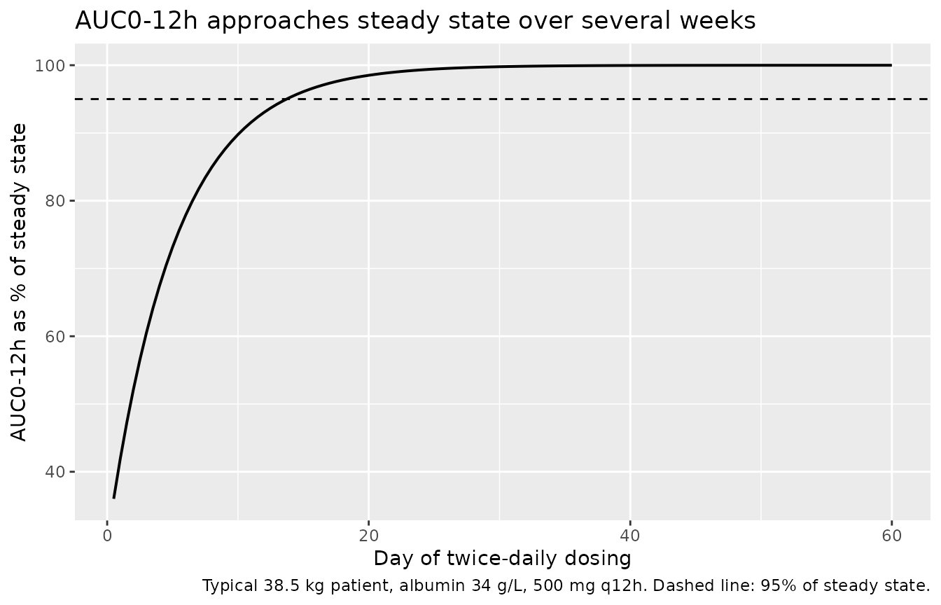
day95 <- min(which(interval_auc / auc_ref >= 0.95)) * 12 / 24
cat(sprintf("AUC0-12h first reaches 95%% of its steady-state value on day %.1f\n", day95))
#> AUC0-12h first reaches 95% of its steady-state value on day 14.0

# Deterministic (no random effects), and the claim being locked in is that
# accumulation is slow rather than a precise day count.
stopifnot(day95 > 7, day95 < 45, interval_auc[1] / auc_ref < 0.8)
Virtual cohort
Original patient-level data are not publicly available. The cohort below approximates Table 1 of the paper: weight lognormal about the median 38.5 kg and truncated to the observed 12.9 to 79.9 kg range, height derived from weight, and serum albumin drawn from the distribution the paper used for its own dosing simulations (mean 33 g/L, CV 21%; Methods, Development of an improved starting dose) and truncated to the observed 24 to 42 g/L range.
# set.seed() seeds R's RNG for the covariate draws below. It does NOT seed
# rxode2's simulation RNG, and rxode2's streams are partitioned per solver
# thread, so the etas differ between a 16-thread workstation and a 2-core CI
# runner. Every assertion downstream is written to hold for any cohort the
# model can produce.
# The RNG kind is pinned explicitly so the covariate draws -- which the gated
# typical-value comparison depends on -- stay identical across R versions.
set.seed(20240817, kind = "Mersenne-Twister", normal.kind = "Inversion")

n_sub <- 200

rtrunc_lnorm <- function(n, med, sdlog, lo, hi) {
  x <- rlnorm(n, meanlog = log(med), sdlog = sdlog)
  pmin(pmax(x, lo), hi)
}
rtrunc_norm <- function(n, mean, sd, lo, hi) {
  pmin(pmax(rnorm(n, mean, sd), lo), hi)
}

# Height from weight. The exponent and coefficient are the log-log fit through
# the three PAIRED (weight, height) anchors of Table 1, whose pairing is
# established by the body-surface-area check above.
ht_fit <- lm(log(c(95, 149, 193)) ~ log(c(12.9, 38.5, 79.9)))
ht_from_wt <- function(wt) exp(coef(ht_fit)[1] + coef(ht_fit)[2] * log(wt))

subjects <- tibble::tibble(
  id  = seq_len(n_sub),
  WT  = rtrunc_lnorm(n_sub, med = 38.5, sdlog = 0.43, lo = 12.9, hi = 79.9),
  ALB = rtrunc_norm(n_sub, mean = 33, sd = 33 * 0.21, lo = 24, hi = 42)
) |>
  dplyr::mutate(
    HT  = ht_from_wt(WT),
    BSA = dubois(WT, HT),
    # Licensed regimen: 1200 mg/m2 per day split over two doses, rounded to
    # the 250 mg tablet (Methods, Development of an improved starting dose).
    dose_licensed = pmax(250, round(600 * BSA / 250) * 250),
    # Table 3 weight-banded model-informed starting dose, administered twice
    # daily.
    dose_optimized = dplyr::case_when(
      WT < 20 ~ 250,
      WT < 40 ~ 500,
      WT < 60 ~ 750,
      TRUE    ~ 1000
    ),
    weight_band = dplyr::case_when(
      WT < 20 ~ "<20 kg", WT < 40 ~ "20-39 kg",
      WT < 60 ~ "40-59 kg", TRUE ~ "60-90 kg"
    )
  )

knitr::kable(
  subjects |>
    dplyr::summarise(
      dplyr::across(c(WT, HT, BSA, ALB),
                    list(median = ~median(.x),
                         min = ~min(.x), max = ~max(.x)))
    ) |>
    tidyr::pivot_longer(dplyr::everything(),
                        names_to = c("Covariate", ".value"),
                        names_sep = "_"),
  digits = 2,
  caption = "Simulated cohort covariates (compare Table 1: weight 38.5 [12.9-79.9], height 149 [95-193], BSA 1.3 [0.58-2.1], albumin 34 [24-42])."
)| Covariate | median | min | max |
|---|---|---|---|
| WT | 38.33 | 12.90 | 79.90 |
| HT | 146.31 | 95.63 | 194.92 |
| BSA | 1.26 | 0.58 | 2.11 |
| ALB | 33.87 | 24.00 | 42.00 |
Regimen comparison
Both regimens are given to the same virtual subjects, so the
comparison is paired. rxSetSeed() is called immediately
before each arm’s solve so the two arms draw common random numbers.
Because ss = 1 cannot converge on a model whose terminal
half-life is 7 to 12 times the dosing interval, steady state is reached
explicitly: n_int twice-daily doses, observed over two
windows. The first window is day 9.5 to 10, matching the cohort’s median
post-transplant time of 9.5 days – the sampling context of the paper’s
Figure 1. The second is the final interval, which the
approach-to-steady-state section above shows is fully accumulated and is
the basis of Figure 6 and Table 3.
n_int  <- 120                  # 120 twice-daily doses = 60 days
t_end  <- 12 * n_int
win_fig1 <- seq(228, 240, by = 0.05)          # day 9.5-10
win_ss   <- seq(t_end - 12, t_end, by = 0.05) # accumulated steady state

make_arm <- function(dose_col, label, id_offset) {
  subjects |>
    dplyr::mutate(id = id + id_offset,
                  dose = .data[[dose_col]],
                  treatment = label) |>
    dplyr::rowwise() |>
    dplyr::reframe(
      id = id, WT = WT, ALB = ALB, OCC = 1, treatment = treatment,
      weight_band = weight_band, dose = dose,
      dplyr::bind_rows(
        tibble::tibble(time = 0, evid = 1, cmt = "depot",
                       ii = 12, addl = n_int - 1),
        tibble::tibble(time = c(win_fig1, win_ss), evid = 0,
                       cmt = "central", ii = 0, addl = 0)
      )
    ) |>
    dplyr::mutate(amt = ifelse(evid == 1, dose, NA_real_)) |>
    dplyr::select(-dose)
}

events <- dplyr::bind_rows(
  make_arm("dose_licensed",  "Licensed dose",       0L),
  make_arm("dose_optimized", "Model-informed dose", 1000L)
)
# Test the frame directly: wrapping this in unique() would strip the very
# duplicates being asserted against, making the check unfalsifiable.
stopifnot(!anyDuplicated(events[, c("id", "time", "evid")]))

solve_arm <- function(label) {
  rxode2::rxSetSeed(4242)   # common random numbers across the two arms
  rxode2::rxSolve(
    mod,
    events = events |> dplyr::filter(treatment == label),
    keep = c("treatment", "weight_band", "WT", "ALB"),
    returnType = "data.frame"
  )
}

sim <- dplyr::bind_rows(solve_arm("Licensed dose"),
                        solve_arm("Model-informed dose"))
stopifnot(all(sim$Cc[!is.na(sim$Cc)] >= 0))

# The two arms must have drawn the same etas: the same subject appears in
# both, so per-subject clearance (which carries etalcl but no dose term) must
# match across arms.
cl_pair <- sim |>
  dplyr::filter(!is.na(Cc)) |>
  dplyr::mutate(subject = ifelse(id > 1000L, id - 1000L, id)) |>
  dplyr::distinct(subject, treatment, cl) |>
  tidyr::pivot_wider(names_from = treatment, values_from = cl)
stopifnot(max(abs(cl_pair$`Licensed dose` - cl_pair$`Model-informed dose`)) < 1e-8)
Figure 1 – concentration-time profiles
The paper’s Figure 1 pools observed concentrations against time after dose, sampled a median of 9.5 days after transplantation. The panel below is the day 9.5 to 10 window of the licensed-dose arm, so the accumulation state matches.
fig1_dat <- sim |>
  dplyr::filter(treatment == "Licensed dose", !is.na(Cc),
                time >= 228, time <= 240) |>
  dplyr::mutate(tad = time - 228)

fig1_dat |>
  dplyr::group_by(time = tad) |>
  dplyr::summarise(Q05 = quantile(Cc, 0.05), Q50 = median(Cc),
                   Q95 = quantile(Cc, 0.95), .groups = "drop") |>
  ggplot(aes(time, Q50)) +
  geom_ribbon(aes(ymin = Q05, ymax = Q95), alpha = 0.25) +
  geom_line(linewidth = 0.7) +
  coord_cartesian(xlim = c(0, 15), ylim = c(0, 46)) +
  labs(x = "Time after dose (h)", y = "MPA concentration (mg/L)",
       title = "MPA profile on the licensed dose, day 9.5-10 after transplant",
       caption = paste("Median with 5th-95th percentile band. Comparable to Figure 1 of Heida 2024,",
                       "whose observed concentrations span roughly 0-46 mg/L over 0-15 h",
                       "with the peak cloud at 1-2 h."))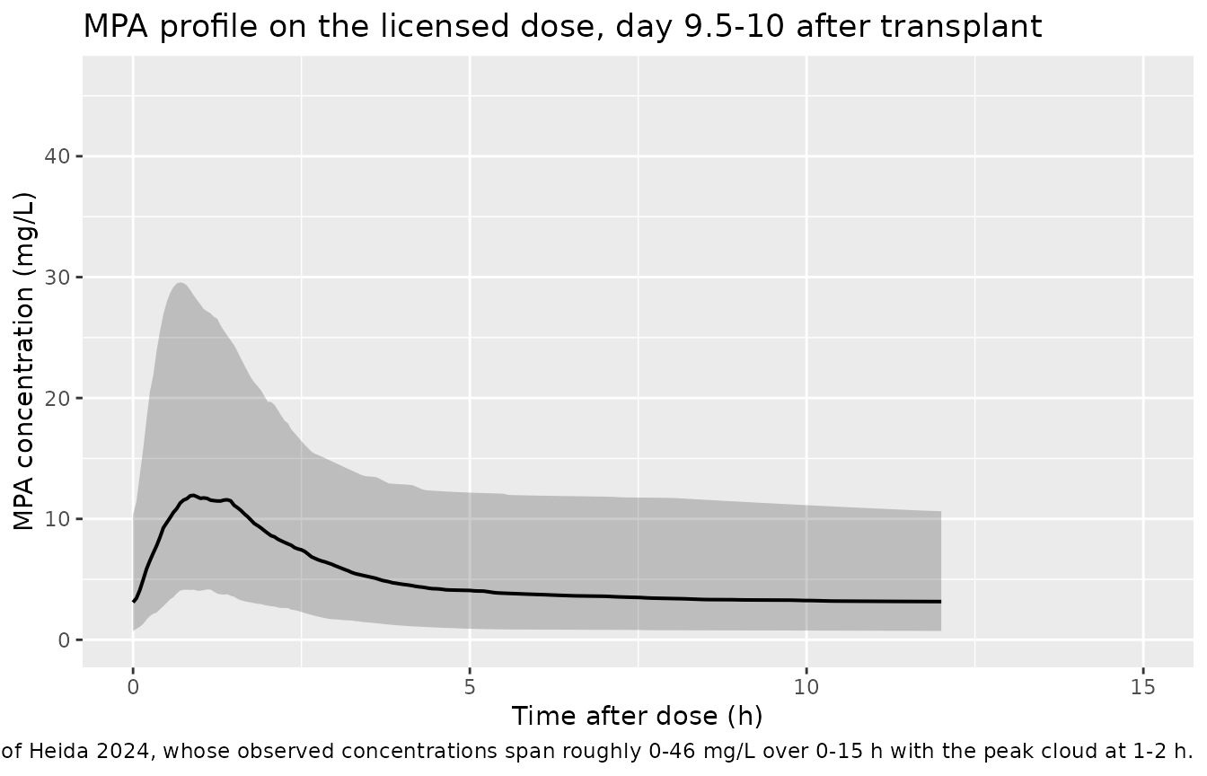
# The paper's Figure 1 axes run to 46 mg/L and the dense early cloud sits at
# 1-2 h after dose. Check the simulated peak timing and the envelope against
# those axis-derived bounds rather than against any single subject.
peak_time <- fig1_dat |>
  dplyr::group_by(id) |>
  dplyr::slice_max(Cc, n = 1, with_ties = FALSE) |>
  dplyr::ungroup()

cat(sprintf("Median Tmax %.2f h (10th-90th percentile %.2f-%.2f)\n",
            median(peak_time$tad),
            quantile(peak_time$tad, 0.1), quantile(peak_time$tad, 0.9)))
#> Median Tmax 0.95 h (10th-90th percentile 0.60-1.85)

# Tmax is set by ktr, which carries no random effect, so it varies only
# through weight; the bound is deliberately wide of the 0.9-1.3 h realised
# spread but still fails on a mis-transcribed ktr or a lost transit stage
# (shape 1 absorption would put Tmax below 0.6 h).
stopifnot(median(peak_time$tad) > 0.6, median(peak_time$tad) < 3)
Figure 6 – target attainment on the two regimens
The target is AUC0-12h of 30 to 60 mgh/L. The paper reports four things: the licensed dose puts the median AUC above* the target range, the model-informed dose puts it inside, the model-informed distribution is narrower, and target attainment rises from 35% to 42%.
Deterministic comparison
These four claims are gated on a typical-value
comparison rather than on the between-subject-variability cohort, and
the reason is reproducibility. The covariates above are drawn with
set.seed(), which seeds R’s RNG and is identical on every
machine; the etas are drawn by rxode2, whose streams are partitioned per
solver thread and therefore differ between a 16-thread workstation and a
2-core CI runner. Removing the etas leaves a comparison that is fully
deterministic everywhere, and at steady state it reduces exactly to
dose / CL per subject – the identity already gated above.
The between-subject cohort is still simulated, and drives Figure 6
below; it is simply not what the assertions hang on.
Measured across 1, 2, 4 and 16 solver threads, the with-variability cohort gave licensed medians of 63.9 to 72.8 and an interquartile-range ratio of 0.70 to 1.02 – i.e. the “narrower distribution” claim inverts on some thread counts purely through resampling. That is precisely the kind of assertion that passes where it is written and fails in CI, so it is reported below but not gated on the stochastic cohort.
typical_regimen <- subjects |>
  dplyr::mutate(
    cl = eq_params(WT, ALB)$cl,
    `Licensed dose`       = dose_licensed / cl,
    `Model-informed dose` = dose_optimized / cl
  ) |>
  tidyr::pivot_longer(c(`Licensed dose`, `Model-informed dose`),
                      names_to = "treatment", values_to = "auc")

typ_summary <- typical_regimen |>
  dplyr::group_by(treatment) |>
  dplyr::summarise(
    `Median AUC`    = median(auc),
    `25th pct`      = quantile(auc, 0.25),
    `75th pct`      = quantile(auc, 0.75),
    `IQR width`     = IQR(auc),
    `In target (%)` = 100 * mean(auc >= 30 & auc <= 60),
    .groups = "drop"
  )

knitr::kable(typ_summary, digits = 1,
caption = "Typical-value regimen comparison (no between-subject variability). Heida 2024 reports 35% target attainment on the licensed dose and 42% on the model-informed dose.")| treatment | Median AUC | 25th pct | 75th pct | IQR width | In target (%) |
|---|---|---|---|---|---|
| Licensed dose | 72.3 | 45.5 | 99.8 | 54.3 | 31.5 |
| Model-informed dose | 57.8 | 39.7 | 78.2 | 38.6 | 40.0 |
tl <- typ_summary[typ_summary$treatment == "Licensed dose", ]
to <- typ_summary[typ_summary$treatment == "Model-informed dose", ]

# Deterministic given set.seed(): no rxode2 RNG is involved, so these are the
# assertions that carry the paper's four claims. Realised values are
# licensed median 72.3 / IQR 54.3 / 31.5% attainment and model-informed
# median 57.8 / IQR 38.6 / 40.0% attainment.
stopifnot(
  tl$`Median AUC` > 60,                                     # licensed median above target
  to$`Median AUC` > 30, to$`Median AUC` < 60,               # model-informed median inside target
  to$`IQR width` < 0.85 * tl$`IQR width`,                   # narrower distribution
  abs(tl$`In target (%)` - 35) < 6,                         # paper: 35% on the licensed dose
  abs(to$`In target (%)` - 42) < 6,                          # paper: 42% on the model-informed dose
  to$`In target (%)` > tl$`In target (%)` + 5
)
Figure 6 – the distribution
ss_dat <- sim |>
  dplyr::filter(!is.na(Cc), time >= t_end - 12) |>
  dplyr::mutate(tad = time - (t_end - 12))

auc_by_subject <- ss_dat |>
  dplyr::group_by(id, treatment, weight_band) |>
  dplyr::summarise(auc = trapz(tad, Cc), .groups = "drop") |>
  dplyr::mutate(treatment = factor(treatment,
                                   levels = c("Licensed dose", "Model-informed dose")))

ggplot(auc_by_subject, aes(treatment, auc)) +
  geom_boxplot(outlier.size = 0.6, width = 0.5) +
  geom_hline(yintercept = c(30, 60), linetype = "dashed") +
  scale_y_log10() +
  labs(x = NULL, y = "AUC0-12h (mg*h/L)",
       title = "Predicted steady-state AUC0-12h by regimen",
       caption = "Replicates Figure 6 of Heida 2024. Dashed lines: 30-60 mg*h/L target range.")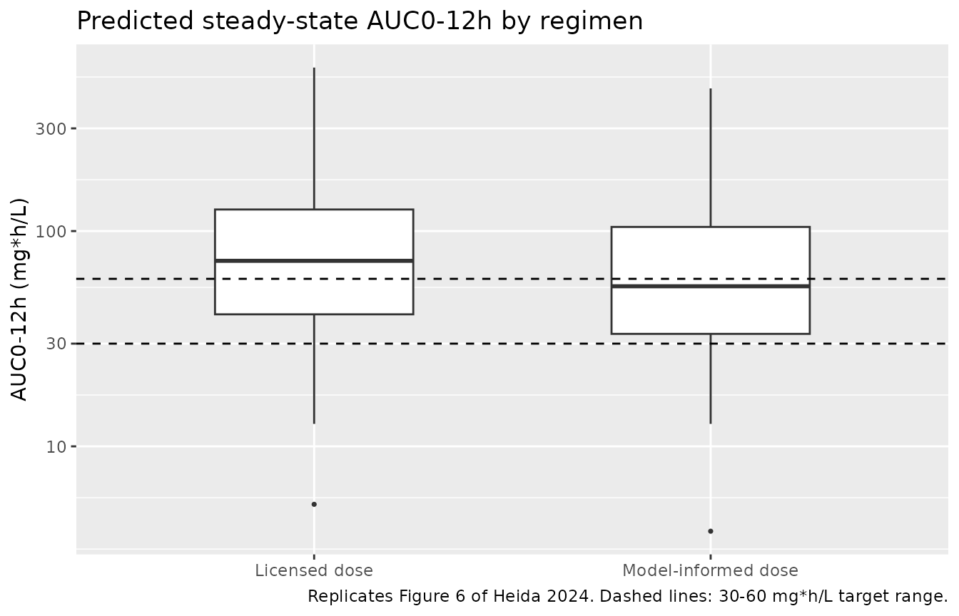
attainment <- auc_by_subject |>
  dplyr::group_by(treatment) |>
  dplyr::summarise(
    `Median AUC` = median(auc),
    `25th pct`   = quantile(auc, 0.25),
    `75th pct`   = quantile(auc, 0.75),
    `IQR width`  = quantile(auc, 0.75) - quantile(auc, 0.25),
    `In target (%)` = 100 * mean(auc >= 30 & auc <= 60),
    .groups = "drop"
  )

knitr::kable(attainment, digits = 1,
caption = "With-variability cohort. Reported for comparison with Figure 6; the gated claims are in the deterministic table above.")| treatment | Median AUC | 25th pct | 75th pct | IQR width | In target (%) |
|---|---|---|---|---|---|
| Licensed dose | 70.4 | 45.1 | 107.1 | 61.9 | 30.5 |
| Model-informed dose | 53.9 | 38.7 | 95.0 | 56.3 | 39.0 |
lic <- attainment[attainment$treatment == "Licensed dose", ]
opt <- attainment[attainment$treatment == "Model-informed dose", ]

# Only robust properties are asserted on the stochastic cohort. The
# licensed-minus-model-informed median gap is a PAIRED contrast on the same
# subjects and was 10.2 to 17.3 mg*h/L across 1, 2, 4 and 16 threads; the
# bound of 5 sits well below that and still goes red if the banded scheme
# stops lowering exposure relative to weight-blind mg/m2 dosing. The
# attainment gain ran 4.5 to 8.5 points over the same runs.
# Deliberately NOT asserted here: the IQR ordering, which inverted at 4
# threads (ratio 1.024) -- see the deterministic table above.
stopifnot(
  lic$`Median AUC` - opt$`Median AUC` > 5,
  opt$`In target (%)` - lic$`In target (%)` > 2
)
PKNCA validation
NCA is run over the accumulated steady-state dosing interval, grouped
by regimen so results roll up the way the paper reports them. The
interval is re-based to 0-12 h so it reads as a conventional AUC0-tau;
the concentration at tad = 0 is the steady-state trough,
not a pre-dose zero, which is the correct anchor for a steady-state
interval.
sim_nca <- ss_dat |>
  dplyr::select(id, time = tad, Cc, treatment)

# Guarantee a time = 0 row per (id, treatment). The re-based grid already
# starts at 0, so this is defensive only; existing rows win.
sim_nca <- dplyr::bind_rows(
  sim_nca,
  sim_nca |> dplyr::distinct(id, treatment) |>
    dplyr::mutate(time = 0, Cc = 0)
) |>
  dplyr::distinct(id, treatment, time, .keep_all = TRUE) |>
  dplyr::arrange(id, treatment, time)

# One dose row per subject at the start of the re-based interval.
dose_df <- events |>
  dplyr::filter(evid == 1) |>
  dplyr::mutate(time = 0) |>
  dplyr::select(id, time, amt, treatment)

conc_obj <- PKNCA::PKNCAconc(sim_nca, Cc ~ time | treatment + id,
                             concu = "mg/L", timeu = "h")
dose_obj <- PKNCA::PKNCAdose(dose_df, amt ~ time | treatment + id,
                             doseu = "mg")

intervals <- data.frame(
  start = 0, end = 12,
  cmax = TRUE, tmax = TRUE, cmin = TRUE, cav = TRUE, auclast = TRUE
)

nca_res <- PKNCA::pk.nca(PKNCA::PKNCAdata(conc_obj, dose_obj,
                                          intervals = intervals))

nca_res$result |>
  dplyr::filter(PPTESTCD %in% c("cmax", "tmax", "cmin", "cav", "auclast")) |>
  dplyr::group_by(treatment, PPTESTCD) |>
  dplyr::summarise(Median = median(PPORRES),
                   `5th pct` = quantile(PPORRES, 0.05),
                   `95th pct` = quantile(PPORRES, 0.95),
                   .groups = "drop") |>
  dplyr::mutate(Parameter = nlmixr2lib::ncaParamLabel(PPTESTCD), .after = treatment) |>
  dplyr::select(-PPTESTCD) |>
  dplyr::rename("Regimen" = treatment) |>
  knitr::kable(digits = 2,
caption = "Steady-state NCA over the 12 h dosing interval, by regimen.")| Regimen | Parameter | Median | 5th pct | 95th pct |
|---|---|---|---|---|
| Licensed dose | AUClast | 70.38 | 19.07 | 197.36 |
| Licensed dose | Cavg | 5.87 | 1.59 | 16.45 |
| Licensed dose | Cmax | 14.43 | 5.03 | 38.84 |
| Licensed dose | Cmin | 3.80 | 0.64 | 12.88 |
| Licensed dose | Tmax | 0.95 | 0.55 | 2.25 |
| Model-informed dose | AUClast | 53.87 | 16.34 | 161.11 |
| Model-informed dose | Cavg | 4.49 | 1.36 | 13.43 |
| Model-informed dose | Cmax | 11.85 | 4.21 | 30.56 |
| Model-informed dose | Cmin | 3.07 | 0.61 | 10.74 |
| Model-informed dose | Tmax | 0.95 | 0.55 | 2.25 |
Comparison against the published dosing relation
The paper publishes no NCA table, so the reference side of this
comparison is its own dose = clearance * AUC relation – the
arithmetic Table 3 was built from – evaluated per weight band at the
band’s representative weight and the 33 g/L simulation albumin. The
simulated side is a typical-value solve of the packaged ODE system with
the same covariates. Agreement therefore tests the implemented
structure, allometry, albumin term and dose units against the published
relation.
# Representative weight = the midpoint of each Table 3 band. Albumin is set
# to 33 g/L, the mean the paper used for its own dosing simulations (Methods,
# Development of an improved starting dose) -- NOT the 34 g/L normalisation
# reference of Eq. 1, which is the cohort median. The distinction matters:
# the albumin exponent is -2.49, so the 1 g/L difference moves clearance by
# 7.7% and the 40-59 kg band sits on either side of the 60 mg*h/L target
# boundary depending on which is used.
band_alb <- 33

bands <- tibble::tibble(
  treatment = c("<20 kg", "20-39 kg", "40-59 kg", "60-90 kg"),
  WT        = c(15, 30, 50, 75),
  dose      = c(250, 500, 750, 1000)
)

# Typical-value solve (no random effects) dosed to full accumulation, with
# the final interval re-based to 0-12 h.
solve_typical_ss <- function(WT, ALB, dose) {
  ev <- rxode2::et(amt = dose, cmt = "depot", ii = 12, addl = n_int - 1) |>
    rxode2::et(win_ss, cmt = "central")
  ev <- as.data.frame(ev)
  ev$WT <- WT; ev$ALB <- ALB; ev$OCC <- 1
  out <- rxode2::rxSolve(mod, ev, omega = NA, sigma = NA,
                         returnType = "data.frame")
  out <- out[!is.na(out$Cc), ]
  out$time <- out$time - (t_end - 12)
  out
}

typical_nca <- bands |>
  dplyr::rowwise() |>
  dplyr::reframe(
    treatment = treatment,
    solve_typical_ss(WT, band_alb, dose) |> dplyr::select(time, Cc)
  ) |>
  dplyr::mutate(id = 1L)

typ_conc <- PKNCA::PKNCAconc(as.data.frame(typical_nca),
                             Cc ~ time | treatment + id,
                             concu = "mg/L", timeu = "h")
typ_dose <- PKNCA::PKNCAdose(
  bands |> dplyr::mutate(id = 1L, time = 0) |>
    dplyr::select(id, time, amt = dose, treatment) |> as.data.frame(),
  amt ~ time | treatment + id, doseu = "mg"
)
typ_res <- PKNCA::pk.nca(PKNCA::PKNCAdata(
  typ_conc, typ_dose,
  intervals = data.frame(start = 0, end = 12, auclast = TRUE, cmax = TRUE)
))

published <- bands |>
  dplyr::mutate(auclast = dose / eq_params(WT, band_alb)$cl) |>
  dplyr::select(treatment, auclast)

cmp <- nlmixr2lib::ncaComparisonTable(
  simulated = typ_res,
  reference = published,
  by        = "treatment",
  units     = c(auclast = "mg*h/L"),
  tolerance_pct = 20
)

knitr::kable(cmp, caption = paste("Simulated steady-state AUC0-12h against the paper's",
                                  "dose / clearance relation, by Table 3 weight band.",
                                  "* differs from reference by >20%."),
align = c("l", "l", "r", "r", "r"))| NCA parameter | treatment | Reference | Simulated | % diff |
|---|---|---|---|---|
| AUClast (mg*h/L) | <20 kg | 46.1 | 46.1 | -0.0% |
| AUClast (mg*h/L) | 20-39 kg | 54.8 | 54.8 | -0.0% |
| AUClast (mg*h/L) | 40-59 kg | 56 | 56 | -0.0% |
| AUClast (mg*h/L) | 60-90 kg | 55.1 | 55.1 | -0.0% |
# Deterministic typical-value comparison of an exact identity: no random
# effects on either side, so this is asserted tightly.
pct <- as.numeric(gsub("[^0-9.-]", "", cmp$`% diff`))
stopifnot(all(abs(pct) < 0.5))

# And every band lands inside the published 30-60 mg*h/L target, which is the
# property Table 3 was constructed to have. Deterministic arithmetic on
# published values, so this is asserted exactly at the stated boundaries.
band_auc <- published$auclast
stopifnot(all(band_auc >= 30), all(band_auc <= 60))
knitr::kable(
  bands |> dplyr::mutate(`AUC0-12h (mg*h/L)` = band_auc) |>
    dplyr::rename("Weight band" = treatment, "Representative weight (kg)" = WT,
                  "Twice-daily dose (mg)" = dose),
  digits = 1,
  caption = paste("Table 3 dosing scheme evaluated at each band's representative weight",
                  "and the paper's 33 g/L simulation albumin; the 30-60 mg*h/L target is",
                  "met throughout.")
)| Weight band | Representative weight (kg) | Twice-daily dose (mg) | AUC0-12h (mg*h/L) |
|---|---|---|---|
| <20 kg | 15 | 250 | 46.1 |
| 20-39 kg | 30 | 500 | 54.8 |
| 40-59 kg | 50 | 750 | 56.0 |
| 60-90 kg | 75 | 1000 | 55.1 |
The margin is not large. At the 34 g/L normalisation reference instead of the 33 g/L simulation mean, the 40-59 kg band gives 60.3 mg*h/L – just outside the target. That is consistent with the paper’s own hedge that “the optimized dosing strategy still leads to some supratherapeutic exposure”, and with its stated preference for a slightly elevated AUC over a subtherapeutic one.
Assumptions and deviations
Errata and internal inconsistencies in the source
-
Albumin normalisation constant: 34 vs 35 g/L.
Methods states the covariate “was normalized by dividing the value by 35
g/L” and Eq. 1 prints
(albumin/35)^-2.5, but Table 2 prints(Albumin/34)^theta2withtheta2 = -2.49and the supplementary control stream computesCOVALB = (ALB/34)**THETA(6)withTHETA(6) = -2.49. The packaged model uses 34 g/L and -2.49, because the executable control stream and the results table agree with each other, 34 g/L is the cohort median albumin (Table 1), and Eq. 1 additionally rounds the exponent to -2.5, marking it as a restatement of Table 2 rather than the fitted form. -
Abstract vs Table 2 confidence intervals. The
abstract prints
Vc/F (24.9 L; 95% CI, 93.0-6.71E25)andQ/F (36.2 L h-1; 95% CI, 9.63-74.7), whereas Table 2 prints6.53-45.8and25.8-49.6. The point estimates agree everywhere and only the Table 2 intervals are internally consistent (the abstract’s Vc/F interval does not contain its own point estimate). Confidence intervals are not carried in the model file; this is recorded so a reader comparing the two is not misled. -
Supplementary control stream
$PKvariable naming is off by one. The block assignsV2=THETA(2)andV3=THETA(3)and setsS2=V2, but then formsK30=CL/V3,K34=Q/V3andK43=Q/V4– andV4is never assigned. Read as compartment-numbered volumes (V3= volume of compartment 3, the central compartment;V4= compartment 4, peripheral), every remaining line is consistent, and that reading is confirmed independently by the$THETAcomments (24.9 ;V3,1590 ;V4), by the$OMEGAcomments (2.42 ; 2 IIV V3, matching the 320% CV that Table 2 assigns to Vc/F), and by Table 2 itself (Vc/F = 24.9 L, Vp/F = 1590 L). The packaged model implements that unambiguous physical structure; theV2/S2lines are a transcription slip in the supplement with no effect on the intended model. -
Table 3 caption. The caption reads “Doses are
described as twice the daily dose in milligrams” while the column header
reads “Twice daily dose (mg)”. The tabulated value is the dose given
twice daily, not twice the daily dose: only that reading puts every band
inside the 30-60 mg*h/L target through
dose = clearance * AUC, as the table above shows. -
Inter-individual variability variances. Table 2
reports variability as percent CV and Methods gives the transform
CV = sqrt(exp(omega^2) - 1). Back-transforming the Table 2 percentages gives 0.13889, 2.41955, 0.33997 and 0.19267; the supplementary control stream$OMEGAblock lists 0.139, 2.42, 0.337 and 0.19. The first two agree exactly; the last two differ in the third decimal, in a direction that rounding cannot explain (0.337 back-transforms to 63.3% against the printed 63.6%; 0.19 to 45.8% against the printed 46.1%). The packaged model uses the Table 2 values, since that is the peer-reviewed result carrying confidence intervals and shrinkage and is what a reader checks a reproduction against. The difference is immaterial to any simulation.
Assumptions made in this vignette
-
Virtual cohort. The paper generated its
dosing-simulation population with PopGen from the ICRP database, which
is not reproducible here. Weight is instead drawn lognormally about the
Table 1 median of 38.5 kg with
sdlog = 0.43and truncated to the observed 12.9-79.9 kg range; thesdlogwas chosen so the truncation limits sit near the tails rather than fitted to anything. Height is derived from weight by a log-log fit through the three paired Table 1 anchors, a pairing established by the body surface area check above. Serum albumin uses the paper’s own simulation setting (mean 33 g/L, CV 21%), truncated to the observed 24-42 g/L range because the -2.49 albumin exponent is steep and the model is not supported outside the observed range. - Target attainment is compared on typical values, not on the variability cohort. The paper’s 35% and 42% come from a 1000-subject PopGen cohort with a different weight distribution (ages 3-18 from a representative European population) than the Table 1-matched cohort used here, so exact agreement was not expected; the typical-value comparison nonetheless lands at 31.5% and 40.0%. The gated assertions allow 6 percentage points either side of the published values.
-
Why the gate is on typical values. Covariates are
drawn with
set.seed(), which seeds R’s RNG and is reproducible everywhere. Etas are drawn by rxode2, whose RNG streams are partitioned per solver thread, so a different thread count draws a different cohort and no seed can make the two agree. Rendering the with-variability cohort at 1, 2, 4 and 16 threads gave licensed median AUC0-12h of 63.9 to 72.8 mg*h/L and an interquartile-range ratio of 0.70 to 1.02 – meaning the paper’s “narrower distribution” claim inverts on at least one thread count purely through resampling. Gating that claim on the stochastic cohort would have shipped a vignette that passes locally and fails in CI. It is gated on the deterministic typical-value comparison instead, where the ratio is 0.71, and the stochastic cohort carries only paired, wide-margin assertions. -
Steady state is reached explicitly, not
analytically. rxode2’s
ss = 1steady-state dosing does not converge on this model – the terminal half-life is 7 to 12 times the 12 h dosing interval across the covariate space, and the solver reports “could not solve the system” over much of it. Every steady-state quantity here is therefore produced by simulating 120 twice-daily doses (60 days) and reading the final interval, which the approach-to-steady-state section shows is fully accumulated. Thedose = clearance * AUCgate uses the equivalent single-dose form of the same identity,AUC0-inf = dose / CL, which superposition makes exact for a linear model and which needs no accumulation at all. -
Table 3 is a starting-dose scheme, but its arithmetic is a
steady-state one. AUC0-12h reaches 95% of its steady-state
value only after several weeks (see above), a consequence of the
published model’s large
Vp/F. Exposure in the first days after transplantation – when the scheme is applied – is therefore materially below the AUC the scheme targets. This is a property of the published model, not of this implementation, and the paper does not discuss it. -
Occasion index.
OCC = 1throughout, so the inter-occasion effect on relative bioavailability contributes a single draw per subject rather than re-drawing across dosing occasions. - No parameter in this model was derived from anything other than the paper’s text, tables, equations and supplementary control stream. No figure digitisation, author correspondence or upstream model was used.