Remdesivir (Abouellil 2023)
Source:vignettes/articles/Abouellil_2023_remdesivir.Rmd
Abouellil_2023_remdesivir.RmdModel and source
- Citation: Abouellil A, Bilal M, Taubert M, Fuhr U. A population pharmacokinetic model of remdesivir and its major metabolites based on published mean values from healthy subjects. Naunyn Schmiedebergs Arch Pharmacol. 2023;396(1):73-82. doi:10.1007/s00210-022-02292-6
- Description: Six-compartment population PK model for intravenous remdesivir and its two plasma metabolites GS-704277 and GS-441524 in healthy adults (Abouellil 2023). Each analyte has a central and a peripheral compartment. Remdesivir is converted to GS-704277 from both of its compartments (central to central, and peripheral to peripheral); GS-704277 is converted to GS-441524 from its central compartment only; each analyte is also eliminated from its central compartment. States are molar amounts (umol), so doses must be supplied in umol of remdesivir. Fitted in Monolix to digitised MEAN concentration profiles of the Gilead single-ascending-dose study, so the random effects are between-dose-cohort, not between-subject, variability.
- Article (open access): https://doi.org/10.1007/s00210-022-02292-6
- Supplementary material (Figures S1-S4; no parameter tables): https://doi.org/10.1007/s00210-022-02292-6
Remdesivir is an intravenous prodrug. Plasma esterases convert it to the alanine intermediate GS-704277, which is cleaved to the nucleoside monophosphate and dephosphorylated to the nucleoside GS-441524, the long-lived circulating metabolite (Abouellil 2023 Figure S1). Abouellil 2023 fitted all three plasma analytes at once. Each analyte has two compartments. Metabolism runs remdesivir -> GS-704277 -> GS-441524 between the central compartments, and there is a second remdesivir -> GS-704277 conversion between the peripheral compartments (Figure 1).
Population
The data were mean concentration-time profiles from the Gilead phase I single-ascending-dose study of remdesivir in healthy volunteers (Humeniuk et al. 2020), digitised from that publication. Six cohorts received a single 2-h intravenous infusion of 3, 10, 30, 75, 150 or 225 mg. Subjects were healthy men and non-pregnant, non-lactating women aged 18-55 years with a body mass index of 18-30 kg/m^2 (Methods). Abouellil 2023 reports no per-cohort sample size, sex split or other demographics; the Discussion notes the cohort had “a focus on a Hispanic population”. The study also included once-daily 1-h infusions for 7 and 14 days, but the model was fitted to the single-dose cohorts only (Table 2 caption).
Because each cohort contributed one mean profile per analyte, the random effects in Table 2 measure how the mean profiles vary between dose cohorts, not how individuals vary (Methods: “the obtained variability of fixed parameters reflects inter-cohort variabilities rather than inter-individual variability”). The authors note in the Discussion that between-patient variability is probably much larger. They tried to apply the model to a patient with renal impairment and it failed.
Source trace
| Model element | Value | Source |
|---|---|---|
| Structure: 2 compartments per analyte, sequential metabolism, elimination from each central compartment | – | Table 1 (ODEs); Figure 1; Results paragraph 1 |
| Peripheral remdesivir -> peripheral GS-704277 conversion | – | Table 1 (RDV and GS-704277 peripheral equations); Figure 1 caption |
lcl (remdesivir CL) |
18.1 L/h | Table 2 |
lvc (remdesivir Vc) |
4.89 L | Table 2 |
lvp (remdesivir Vp) |
46.5 L | Table 2 |
lq (remdesivir Q) |
13.2 L/h | Table 2 |
lcl_form_gs704277_central (CLmc GS-704277) |
16.9 L/h | Table 2, ‘Central formation clearance’, GS-704277 column |
lcl_form_gs704277_peripheral1 (CLmp GS-704277) |
18.9 L/h | Table 2, ‘Peripheral formation clearance’, GS-704277 column |
lcl_gs704277 |
36.9 L/h | Table 2 |
lvc_gs704277 |
96.4 L | Table 2 |
lvp_gs704277 |
8.64 L | Table 2 |
lq_gs704277 |
0.12 L/h | Table 2 |
lcl_form_gs441524 (CLmc GS-441524) |
50.5 L/h | Table 2, ‘Central formation clearance’, GS-441524 column |
lcl_gs441524 |
4.74 L/h | Table 2 |
lvc_gs441524 |
26.2 L | Table 2 |
lvp_gs441524 |
66.2 L | Table 2 |
lq_gs441524 |
55 L/h | Table 2 |
etalcl |
SD 0.39 (variance 0.1521) | Table 2 (SD in parentheses) |
etalcl_form_gs704277_central |
SD 0.25 (variance 0.0625) | Table 2 |
etalcl_form_gs704277_peripheral1 |
SD 0.53 (variance 0.2809) | Table 2 |
etalcl_gs704277 |
SD 0.31 (variance 0.0961) | Table 2 |
etalcl_form_gs441524 |
SD 0.27 (variance 0.0729) | Table 2 |
etalvc_gs441524 |
SD 0.71 (variance 0.5041) | Table 2 |
etalvp_gs441524 |
SD 0.24 (variance 0.0576) | Table 2 |
Log-normal random effects,
log(theta_i) = log(theta_pop) + eta_i
|
– | Methods equation |
| Residual error: proportional (remdesivir), combined (GS-704277), proportional (GS-441524) | magnitudes not reported, held at 0 | Results paragraph 4; Methods error-model equation |
| Saline flush: 4% of the dose given as a bolus at the end of the 2-h infusion | – | Methods (dosing-record design, not part of
model()) |
| Concentration scale nmol/L; molar 1:1 transfer between moieties | – | Figures 2 and 4 axes; Table 1 (no molecular-weight factor) |
Model structure and units
mod <- rxode2::rxode2(readModelDb("Abouellil_2023_remdesivir"))
#> ℹ parameter labels from comments will be replaced by 'label()'
mod_typ <- rxode2::zeroRe(mod)
The model’s states hold molar amounts (umol). Abouellil 2023 Figures
2 and 4 plot every analyte in nmol/L, and the Table 1 equations move
material between moieties as clearance x concentration with no
molecular-weight factor, so the model runs in molar space. Doses in mg
are converted to umol with the remdesivir molecular weight of 602.58
g/mol (the paper does not print it). The observation variables
Cc, Cc_gs704277 and Cc_gs441524
are in nmol/L.
mw_rdv <- 602.58
mg_to_umol <- function(mg) mg / mw_rdv * 1000

# Single-ascending-dose design of the fitted study: a 2-h infusion of 96% of
# the dose followed by 4% as a bolus at the end of the infusion, which is how
# Abouellil 2023 Methods represent the saline flush.
sad_events <- function(dose_mg, obs_times, flush = TRUE) {
  amt <- mg_to_umol(dose_mg)
  ev <- if (flush) {
    rxode2::et(amt = 0.96 * amt, dur = 2, cmt = "central") |>
      rxode2::et(amt = 0.04 * amt, time = 2, cmt = "central")
  } else {
    rxode2::et(amt = amt, dur = 2, cmt = "central")
  }
  # Three endpoints are declared, so observation rows must name one of them;
  # every observable is returned on every row regardless.
  rxode2::et(ev, obs_times, cmt = "Cc")
}

sad_times <- sort(unique(c(seq(0, 2, by = 0.05), 2 + 1e-4,
                           seq(2.05, 12, by = 0.05), seq(12, 144, by = 0.5))))
sad_doses <- c(3, 10, 30, 75, 150, 225)
Observation rows carry cmt = "Cc". With three declared
endpoints, an observation row on an ODE state is rejected by rxode2.
Cc already has its own endpoint slot, so naming it adds no
compartment and does not renumber the ODE states. The guard below checks
this: the dose must land in central.
sad <- dplyr::bind_rows(lapply(sad_doses, function(d) {
  out <- as.data.frame(rxode2::rxSolve(mod_typ, sad_events(d, sad_times),
                                       returnType = "data.frame"))
  out$dose_mg <- d
  out
}))
#> ℹ omega/sigma items treated as zero: 'etalcl', 'etalcl_form_gs704277_central', 'etalcl_form_gs704277_peripheral1', 'etalcl_gs704277', 'etalcl_form_gs441524', 'etalvc_gs441524', 'etalvp_gs441524'
#> ℹ omega/sigma items treated as zero: 'etalcl', 'etalcl_form_gs704277_central', 'etalcl_form_gs704277_peripheral1', 'etalcl_gs704277', 'etalcl_form_gs441524', 'etalvc_gs441524', 'etalvp_gs441524'
#> ℹ omega/sigma items treated as zero: 'etalcl', 'etalcl_form_gs704277_central', 'etalcl_form_gs704277_peripheral1', 'etalcl_gs704277', 'etalcl_form_gs441524', 'etalvc_gs441524', 'etalvp_gs441524'
#> ℹ omega/sigma items treated as zero: 'etalcl', 'etalcl_form_gs704277_central', 'etalcl_form_gs704277_peripheral1', 'etalcl_gs704277', 'etalcl_form_gs441524', 'etalvc_gs441524', 'etalvp_gs441524'
#> ℹ omega/sigma items treated as zero: 'etalcl', 'etalcl_form_gs704277_central', 'etalcl_form_gs704277_peripheral1', 'etalcl_gs704277', 'etalcl_form_gs441524', 'etalvc_gs441524', 'etalvp_gs441524'
#> ℹ omega/sigma items treated as zero: 'etalcl', 'etalcl_form_gs704277_central', 'etalcl_form_gs704277_peripheral1', 'etalcl_gs704277', 'etalcl_form_gs441524', 'etalvc_gs441524', 'etalvp_gs441524'
sad$dose <- factor(paste(sad$dose_mg, "mg"), levels = paste(sad_doses, "mg"))

stopifnot(
  # The infusion fills `central` (state 1), not an injected endpoint slot.
  all(sad$central[sad$time == 1] > 0),
  # Each moiety's central state has no dose of its own and starts at zero.
  all(sad$central_gs704277[sad$time == 0] == 0),
  all(sad$central_gs441524[sad$time == 0] == 0)
)
Steady-state check of the ODE wiring
During a long constant-rate infusion of remdesivir the model has a closed-form steady state. The remdesivir peripheral compartment loses drug only by conversion to GS-704277. GS-704277 formed in its peripheral compartment must come back to its central compartment before it can be eliminated. GS-441524 is formed only from central GS-704277. So, for infusion rate R (umol/h):
-
Cc_ss = R / (CL + CLmc + Q * CLmp / (Q + CLmp)),Cp_ss = Q * Cc_ss / (Q + CLmp) C704_ss = (CLmc * Cc_ss + CLmp * Cp_ss) / (CL_704 + CLm_441)C441_ss = CLm_441 * C704_ss / CL_441
The check uses typical values and a solve against its own closed form, so the two sides differ only by numerical error and a tight tolerance is correct.
p <- exp(c(
  cl = log(18.1), vc = log(4.89), vp = log(46.5), q = log(13.2),
  clmc = log(16.9), clmp = log(18.9),
  cl704 = log(36.9), clm441 = log(50.5), cl441 = log(4.74)
))
rate <- 10 # umol/h
cc_ss <- rate / (p[["cl"]] + p[["clmc"]] + p[["q"]] * p[["clmp"]] / (p[["q"]] + p[["clmp"]]))
cp_ss <- p[["q"]] * cc_ss / (p[["q"]] + p[["clmp"]])
c704_ss <- (p[["clmc"]] * cc_ss + p[["clmp"]] * cp_ss) / (p[["cl704"]] + p[["clm441"]])
c441_ss <- p[["clm441"]] * c704_ss / p[["cl441"]]

ss_ev <- rxode2::et(amt = rate * 2000, rate = rate, cmt = "central") |>
  rxode2::et(1500, cmt = "Cc")
ss <- as.data.frame(rxode2::rxSolve(mod_typ, ss_ev, returnType = "data.frame",
                                    atol = 1e-10, rtol = 1e-10))
#> ℹ omega/sigma items treated as zero: 'etalcl', 'etalcl_form_gs704277_central', 'etalcl_form_gs704277_peripheral1', 'etalcl_gs704277', 'etalcl_form_gs441524', 'etalvc_gs441524', 'etalvp_gs441524'
ss_tab <- data.frame(
  analyte = c("remdesivir", "GS-704277", "GS-441524"),
  closed_form_nM = 1000 * c(cc_ss, c704_ss, c441_ss),
  simulated_nM = c(ss$Cc, ss$Cc_gs704277, ss$Cc_gs441524)
)
ss_tab$rel_diff <- ss_tab$simulated_nM / ss_tab$closed_form_nM - 1
knitr::kable(ss_tab, digits = c(0, 3, 3, 8))| analyte | closed_form_nM | simulated_nM | rel_diff |
|---|---|---|---|
| remdesivir | 233.798 | 233.798 | 0 |
| GS-704277 | 65.998 | 65.998 | 0 |
| GS-441524 | 703.147 | 703.147 | 0 |
Single-dose profiles (replicates Figure 2 of Abouellil 2023)
Figure 2 overlays each cohort’s own empirical-Bayes fit on that cohort’s mean data. The curves below are the population typical values, with every between-cohort random effect at zero.
sad |>
  dplyr::filter(time <= 12) |>
  tidyr::pivot_longer(c(Cc, Cc_gs704277), names_to = "analyte", values_to = "conc") |>
  dplyr::mutate(analyte = dplyr::recode(analyte, Cc = "Remdesivir",
                                        Cc_gs704277 = "GS-704277")) |>
  ggplot(aes(time, conc, colour = dose)) +
  geom_line() +
  facet_wrap(~analyte, ncol = 1, scales = "free_y") +
  labs(x = "Time (h)", y = "Concentration (nmol/L)", colour = "Dose",
       caption = "Replicates Figure 2 (remdesivir and GS-704277 panels) of Abouellil 2023, typical values.")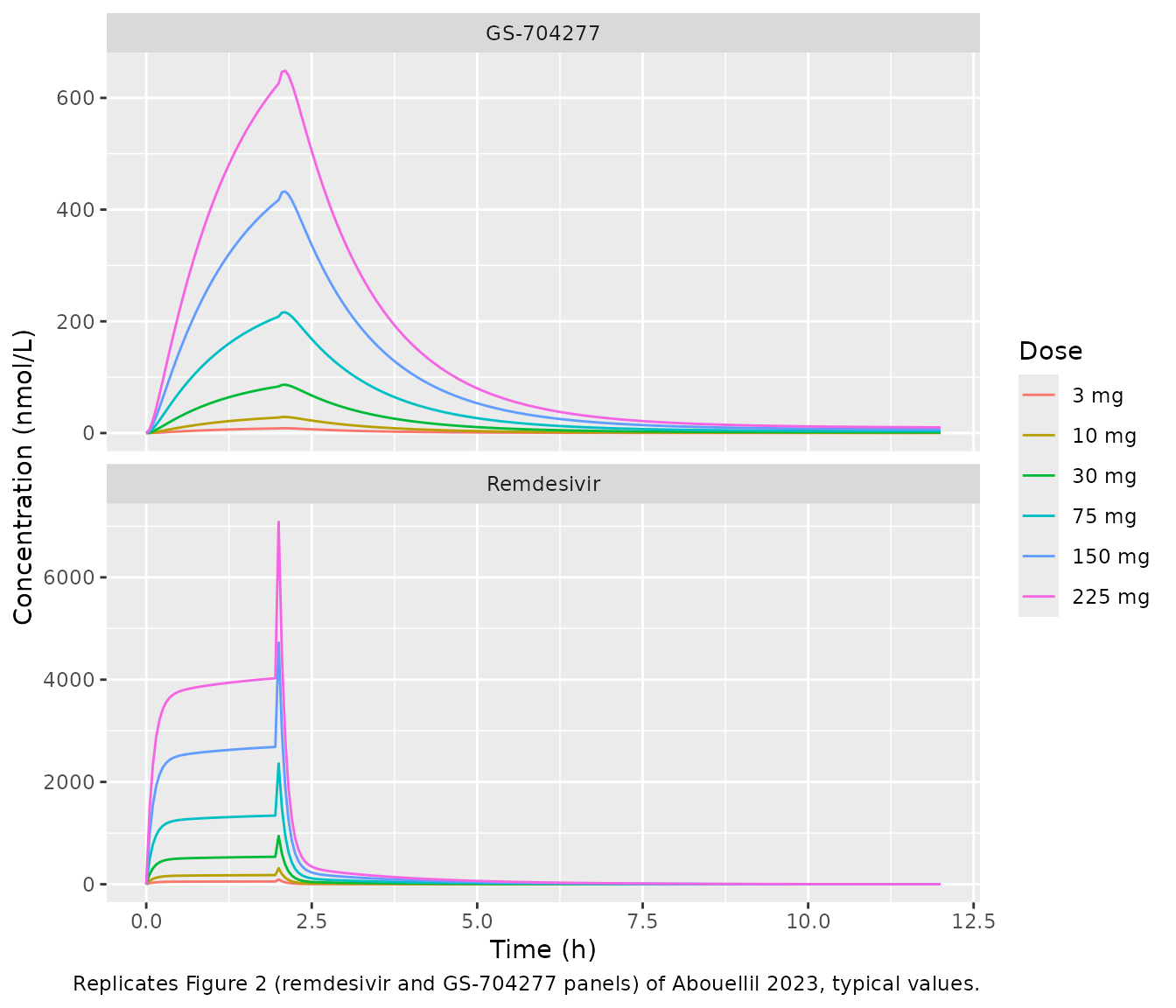
sad |>
  ggplot(aes(time, Cc_gs441524, colour = dose)) +
  geom_line() +
  labs(x = "Time (h)", y = "GS-441524 concentration (nmol/L)", colour = "Dose",
       caption = "Replicates Figure 2 (GS-441524 panels) of Abouellil 2023, typical values.")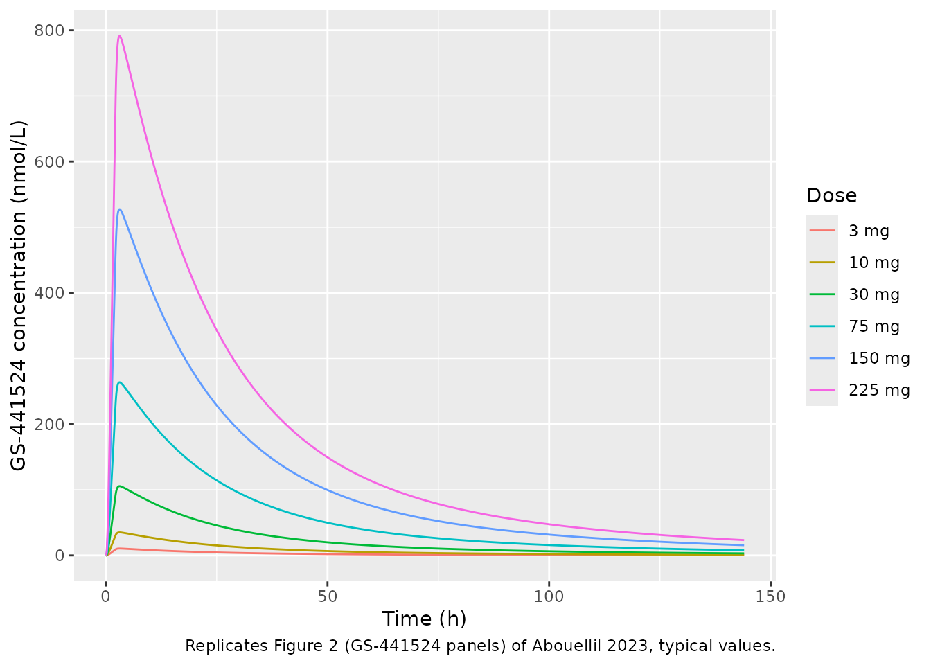
The typical-value peaks are close to the Figure 2 panels. At 225 mg the remdesivir plateau is 3898 nmol/L and the end-of-infusion spike from the flush bolus reaches 7086 nmol/L. GS-704277 peaks at 649 nmol/L and GS-441524 at 791 nmol/L. Figure 2 shows about 3500-4000, 7000, 680 and 850 nmol/L for these four values (read by eye).
Clinical regimen (replicates Figure 4 of Abouellil 2023)
Abouellil 2023 simulated 256 subjects on the licensed regimen: 200 mg as a 30-min infusion on day 1, then 100 mg as a 30-min infusion daily on days 2-5. The simulation sampled the between-cohort random effects (Results: “The simulation used the previously generated population parameters of fixed effects, the standard deviation of the random effects, and error model estimates”). The cohort below uses 200 virtual subjects. The model has no covariates, so the only thing that varies between subjects is the sampled random effects.
rxode2::rxSetSeed(20230101)
n_sub <- 200
clin_times <- sort(unique(c(seq(0, 120, by = 0.1), 0.5 + 24 * 0:4)))
clin_ev <- rxode2::et(amt = mg_to_umol(200), dur = 0.5, cmt = "central") |>
  rxode2::et(amt = mg_to_umol(100), dur = 0.5, time = 24 * 1:4, cmt = "central") |>
  rxode2::et(clin_times, cmt = "Cc") |>
  rxode2::et(id = seq_len(n_sub))
clin <- as.data.frame(rxode2::rxSolve(mod, clin_ev, returnType = "data.frame"))
clin$treatment <- "200 mg LD + 100 mg QD"
stopifnot(!anyNA(clin$Cc), !anyNA(clin$Cc_gs704277), !anyNA(clin$Cc_gs441524),
          length(unique(clin$id)) == n_sub)
clin |>
  tidyr::pivot_longer(c(Cc, Cc_gs704277, Cc_gs441524), names_to = "analyte",
                      values_to = "conc") |>
  dplyr::group_by(analyte, time) |>
  dplyr::summarise(mean = mean(conc), sd = sd(conc), .groups = "drop") |>
  dplyr::mutate(
    analyte = factor(dplyr::recode(analyte, Cc = "Remdesivir",
                                   Cc_gs704277 = "GS-704277",
                                   Cc_gs441524 = "GS-441524"),
                     levels = c("Remdesivir", "GS-704277", "GS-441524")),
    # The pre-dose row is exactly zero; floor it for the log axis.
    mean = pmax(mean, 1e-3), lo = pmax(mean - sd, 1e-3), hi = mean + sd
  ) |>
  ggplot(aes(time, mean)) +
  geom_line() +
  geom_line(aes(y = lo), linetype = "dotted") +
  geom_line(aes(y = hi), linetype = "dotted") +
  scale_y_log10() +
  coord_cartesian(ylim = c(1, NA)) +
  facet_wrap(~analyte, ncol = 1, scales = "free_y") +
  labs(x = "Time (h)", y = "Concentration (nmol/L)",
       caption = "Replicates Figure 4 of Abouellil 2023: mean (solid) +/- SD (dotted).")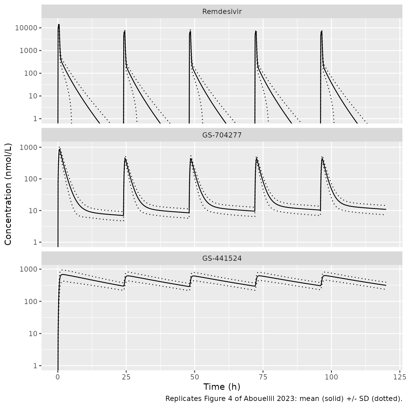
Figure 4 cuts each panel off at the assay LLOQ, and the remdesivir panel adds a fraction-of-censored-observations trace. The LLOQ values come from the source study and are not printed in Abouellil 2023, so neither the cut-off nor the censored-fraction trace is reproduced here. The figure above is drawn down to 1 nmol/L.
Non-compartmental analysis
PKNCA is run on the simulated cohort, once per analyte. The intervals are the first dosing interval (0-24 h, after the 200 mg loading dose) and the last (96-120 h, after the fifth dose).
nca_one <- function(col, label) {
  conc <- clin |>
    dplyr::filter(!is.na(.data[[col]])) |>
    dplyr::transmute(id, time, treatment, conc = .data[[col]])
  dose <- data.frame(id = rep(seq_len(n_sub), each = 5), time = 24 * 0:4,
                     amt = rep(c(200, 100, 100, 100, 100), n_sub),
                     treatment = "200 mg LD + 100 mg QD")
  o_conc <- PKNCA::PKNCAconc(conc, conc ~ time | treatment + id)
  o_dose <- PKNCA::PKNCAdose(dose, amt ~ time | treatment + id)
  intervals <- data.frame(start = c(0, 96), end = c(24, 120),
                          cmax = TRUE, tmax = TRUE, auclast = TRUE)
  res <- PKNCA::pk.nca(PKNCA::PKNCAdata(o_conc, o_dose, intervals = intervals))
  out <- as.data.frame(res)
  out$analyte <- label
  out
}
nca <- dplyr::bind_rows(
  nca_one("Cc", "Remdesivir"),
  nca_one("Cc_gs704277", "GS-704277"),
  nca_one("Cc_gs441524", "GS-441524")
)
nca |>
  dplyr::group_by(analyte, start, end, PPTESTCD) |>
  dplyr::summarise(mean = mean(PPORRES), sd = sd(PPORRES),
                   median = median(PPORRES), .groups = "drop") |>
  dplyr::mutate(interval = paste0(start, "-", end, " h")) |>
  dplyr::select(analyte, interval, PPTESTCD, mean, sd, median) |>
  dplyr::rename("Analyte" = analyte, "Interval" = interval,
                "Parameter" = PPTESTCD, "Mean" = mean, "SD" = sd,
                "Median" = median) |>
knitr::kable(digits = 2)| Analyte | Interval | Parameter | Mean | SD | Median |
|---|---|---|---|---|---|
| GS-441524 | 0-24 h | auclast | 11187.15 | 3649.09 | 10816.55 |
| GS-441524 | 0-24 h | cmax | 712.99 | 269.45 | 673.42 |
| GS-441524 | 0-24 h | tmax | 2.16 | 1.06 | 2.00 |
| GS-441524 | 96-120 h | auclast | 10999.13 | 2765.58 | 11087.36 |
| GS-441524 | 96-120 h | cmax | 645.18 | 180.81 | 637.21 |
| GS-441524 | 96-120 h | tmax | 1.86 | 0.70 | 1.75 |
| GS-704277 | 0-24 h | auclast | 1639.53 | 472.83 | 1605.80 |
| GS-704277 | 0-24 h | cmax | 868.45 | 193.23 | 875.24 |
| GS-704277 | 0-24 h | tmax | 0.62 | 0.04 | 0.60 |
| GS-704277 | 96-120 h | auclast | 1030.14 | 282.09 | 1025.64 |
| GS-704277 | 96-120 h | cmax | 444.44 | 97.49 | 449.07 |
| GS-704277 | 96-120 h | tmax | 0.62 | 0.04 | 0.60 |
| Remdesivir | 0-24 h | auclast | 7775.45 | 1664.18 | 7789.74 |
| Remdesivir | 0-24 h | cmax | 13958.69 | 2426.69 | 14143.83 |
| Remdesivir | 0-24 h | tmax | 0.50 | 0.00 | 0.50 |
| Remdesivir | 96-120 h | auclast | 3887.77 | 832.15 | 3894.87 |
| Remdesivir | 96-120 h | cmax | 6979.36 | 1213.36 | 7071.92 |
| Remdesivir | 96-120 h | tmax | 0.50 | 0.00 | 0.50 |
Comparison against the published simulation results
The Results section reports the cohort-mean Cmax (between-dose SD) after the 200 mg loading dose. The values are 13.7 umol/L (2.39) for remdesivir, 807 nmol/L (173) for GS-704277 and 726 nmol/L (240) for GS-441524. It also reports a GS-441524 Cmax of 645.5 nmol/L (17.57) after the subsequent 100 mg doses. The simulated values below are cohort means of the per-subject PKNCA Cmax, so they are directly comparable.
sim_cmax <- nca |>
  dplyr::filter(PPTESTCD == "cmax") |>
  dplyr::mutate(group = dplyr::case_when(
    start == 0 ~ paste(analyte, "after the 200 mg loading dose"),
    TRUE ~ paste(analyte, "after the fifth (100 mg) dose")
  )) |>
  dplyr::group_by(group) |>
  dplyr::summarise(cmax = mean(PPORRES), .groups = "drop")

ref_cmax <- data.frame(
  group = c("Remdesivir after the 200 mg loading dose",
            "GS-704277 after the 200 mg loading dose",
            "GS-441524 after the 200 mg loading dose",
            "GS-441524 after the fifth (100 mg) dose"),
  cmax = c(13700, 807, 726, 645.5)
)
cmp <- nlmixr2lib::ncaComparisonTable(
  sim_cmax |> dplyr::filter(group %in% ref_cmax$group),
  ref_cmax, by = "group", units = c(cmax = "nmol/L")
)
knitr::kable(cmp)| NCA parameter | group | Reference | Simulated | % diff |
|---|---|---|---|---|
| Cmax (nmol/L) | Remdesivir after the 200 mg loading dose | 13700 | 14000 | +1.9% |
| Cmax (nmol/L) | GS-704277 after the 200 mg loading dose | 807 | 868 | +7.6% |
| Cmax (nmol/L) | GS-441524 after the 200 mg loading dose | 726 | 713 | -1.8% |
| Cmax (nmol/L) | GS-441524 after the fifth (100 mg) dose | 646 | 645 | -0.0% |
pct <- (sim_cmax$cmax[match(ref_cmax$group, sim_cmax$group)] / ref_cmax$cmax - 1) * 100
stopifnot(
  # Cohort means of 200 subjects; a wrong volume, clearance or molar
  # conversion shifts these by far more than the 15% allowed.
  all(abs(pct) < 15)
)
All four simulated means are within 8% of the published values. The GS-704277 loading-dose Cmax is the largest difference (+7.6%). The typical-value GS-704277 Cmax is also above the published mean, so the gap is not only a matter of which 256 subjects were sampled. The paper gives no more detail on its simulation, so the gap is recorded here rather than explained; it is well inside the 20% flag threshold.
Saline flush in the clinical simulation
The 4% end-of-infusion bolus represents the saline flush in the fitted 2-h infusion study. The clinical-regimen simulation above leaves it out. The reported loading-dose remdesivir Cmax of 13.7 umol/L matches the simulation without the flush. With the flush, the bolus lands in a 4.89 L central volume at the moment of peak concentration and raises the typical Cmax by about 2.7 umol/L:
ld <- function(flush) {
  amt <- mg_to_umol(200)
  ev <- if (flush) {
    rxode2::et(amt = 0.96 * amt, dur = 0.5, cmt = "central") |>
      rxode2::et(amt = 0.04 * amt, time = 0.5, cmt = "central")
  } else {
    rxode2::et(amt = amt, dur = 0.5, cmt = "central")
  }
  out <- as.data.frame(rxode2::rxSolve(
    mod_typ, rxode2::et(ev, seq(0, 3, by = 0.01), cmt = "Cc"),
    returnType = "data.frame"
  ))
  max(out$Cc)
}
flush_tab <- data.frame(
  design = c("No flush (used above)", "4% end-of-infusion bolus"),
  typical_cmax_umol_L = c(ld(FALSE), ld(TRUE)) / 1000
)
#> ℹ omega/sigma items treated as zero: 'etalcl', 'etalcl_form_gs704277_central', 'etalcl_form_gs704277_peripheral1', 'etalcl_gs704277', 'etalcl_form_gs441524', 'etalvc_gs441524', 'etalvp_gs441524'
#> ℹ omega/sigma items treated as zero: 'etalcl', 'etalcl_form_gs704277_central', 'etalcl_form_gs704277_peripheral1', 'etalcl_gs704277', 'etalcl_form_gs441524', 'etalvc_gs441524', 'etalvp_gs441524'
flush_tab |>
  dplyr::rename("Design" = design,
                "Typical remdesivir Cmax (umol/L)" = typical_cmax_umol_L) |>
knitr::kable(digits = 2)| Design | Typical remdesivir Cmax (umol/L) |
|---|---|
| No flush (used above) | 13.96 |
| 4% end-of-infusion bolus | 16.12 |
Assumptions and deviations
- Residual error magnitudes are not reported. The Results name the selected error models (proportional for remdesivir, combined for GS-704277, proportional for GS-441524). Neither the paper nor the supplement gives their values. All four residual parameters are held at zero, so simulations have no residual noise. Fit the model to your own data before using it to simulate observed concentrations.
- Random effects are between-cohort, not between-subject. They are variances of the Table 2 SDs (Monolix reports the SD of each random effect). Simulating individuals with them gives a spread of cohort-mean profiles. It will understate the spread of individual patients’ profiles, as the authors point out.
- Molar units and molecular weight. The model is in umol and nmol/L, as Figures 2 and 4 and the molar 1:1 transfer in Table 1 imply. The mg-to-umol conversion uses MW 602.58 g/mol for remdesivir, which the paper does not print. Each metabolite’s clearance and volume are apparent with respect to the unknown fraction of the upstream flux that appears as that metabolite in plasma.
- Saline flush is a dosing-record feature. It is represented in the event table (96% infused, 4% bolus at the end of the infusion) for the 2-h single-dose study, and left out of the 30-min clinical regimen. The reported clinical-regimen remdesivir Cmax supports leaving it out there.
- Assay LLOQs are not available, so the censored-fraction trace of Figure 4 is not reproduced.
- GS-441524 half-life. The Results report a simulated GS-441524 half-life of 29.36 h after repeated 100 mg doses, without saying which window it was fitted over. They also report a regression-based terminal half-life of 20 h from the single-dose data. The model’s terminal phase depends on the window (GS-441524 has a 66.2 L peripheral compartment), so no half-life gate is applied.
Errata and discrepancies in the source
- Table 1, parts of the Methods and the Results text print the intermediate metabolite as “GS-774277”. Table 2, Figure 1, the Abstract and the supplement (Figure S1) give GS-704277, the correct Gilead code. This model uses GS-704277.
- Table 1’s GS-704277 central-compartment equation has an unbalanced parenthesis (“- CL_GS-774277 x Cc_GS-774277)”); the term is read as the GS-704277 elimination outflow.