Semimechanistic antibiotic PD, S. pyogenes time-kill (Nielsen 2007)
Source:vignettes/articles/Nielsen_2007_semimechanistic_antibiotic_pd.Rmd
Nielsen_2007_semimechanistic_antibiotic_pd.RmdModel and source
- Citation: Nielsen EI, Viberg A, Lowdin E, Cars O, Karlsson MO, Sandstrom M. Semimechanistic pharmacokinetic/pharmacodynamic model for assessment of activity of antibacterial agents from time-kill curve experiments. Antimicrob Agents Chemother. 2007;51(1):128-136. doi:10.1128/AAC.00604-06. PMID: 17060524.
- Article: https://doi.org/10.1128/AAC.00604-06
Nielsen and colleagues developed a semi-mechanistic PK/PD model that describes the whole time course of bacterial growth and killing during in-vitro time-kill curve experiments with Streptococcus pyogenes exposed to a wide range of concentrations of five antibiotics with different mechanisms of action: benzylpenicillin (PEN), cefuroxime (CXM), erythromycin (ERY), moxifloxacin (MXF), and vancomycin (VAN). The bacterial system is described with two states – one growing, drug-susceptible population and one resting, drug-insusceptible population – and the drug effect is added to the natural death rate of susceptible bacteria through a sigmoidal Emax function. All 135 experiments were fitted simultaneously in a single NONMEM analysis so that bacterium-specific parameters (kgrowth, kdeath, Bmax) could be separated from drug-specific parameters (Emax, EC50, gamma, ke).
Population
The test organism was Streptococcus pyogenes group A M12 strain NCTC P1800. Time-kill curve experiments were performed in 10 mL glass tubes with 4 mL Todd-Hewitt broth, seeded with a 6-hour logarithmic-growth inoculum of approximately 10^6 CFU/mL, and incubated at 35 C for 24 h with sampling at 0, 1, 2, 4, 6, 9, 12, 15, 18, and 24 h. Antibiotic concentrations tested spanned 0.0625x to 64x MIC for benzylpenicillin, cefuroxime, and erythromycin; 0.25x to 64x MIC for moxifloxacin; and 0.25x to 64x MIC (including 1.5x MIC) for vancomycin. The MICs used in the model were 0.012 mg/L (benzylpenicillin), 0.0313 mg/L (cefuroxime), 0.125 mg/L (erythromycin), 0.125 mg/L (moxifloxacin), and 0.25 mg/L (vancomycin). Each time-kill experiment was performed in duplicate or triplicate on separate occasions with at least one drug-free growth control per day.
The full population metadata is available programmatically via
readModelDb("Nielsen_2007_semimechanistic_antibiotic_pd")()$population.
Source trace
Every parameter carries a source-location comment inline in
inst/modeldb/specificDrugs/Nielsen_2007_semimechanistic_antibiotic_pd.R.
The consolidated trace:
| Element | Value | Source |
|---|---|---|
| Bacterial ODE structure (S, R states) | equations 2, 3 | Materials and Methods p 130 |
| Drug effect equation (equation 4) | sigmoidal Emax | Materials and Methods p 130 |
| Drug effect placement (equation 6) | additive to kdeath | Results p 132 (“in accordance with equation 6”) |
| kSR = (kgrowth - kdeath) * total / Bmax | derivation | Materials and Methods p 130 |
| kRS = 0 | fixed | Materials and Methods p 130 |
| Biophase / effect link | first-order ke | Materials and Methods p 129 (Sheiner 1979 ref 22) |
| kgrowth = 1.35 1/h | typical value | Table 2 |
| kdeath = 0.179 1/h | typical value | Table 2 |
| Bmax = 4.15e8 CFU/mL | typical value | Table 2 |
| fmix1 = 0.747 | typical value | Table 2 |
| fpers = 0.0529 | typical value | Table 2 |
| Benzylpenicillin Emax=2.44, EC50=0.00438, gamma=1.29, ke=1.00 | typical values | Table 3 |
| Cefuroxime Emax=3.30, EC50=0.00829, gamma=1.69, ke=0.861 | typical values | Table 3 |
| Erythromycin Emax=2.03, EC50=0.0276, gamma=0.769, ke=100 (FIX) | typical values | Table 3 |
| Moxifloxacin Emax=3.20, EC50=0.0747, gamma=1.59, ke=0.644 | typical values | Table 3 |
| Vancomycin Emax=1.36, EC50=0.384, gamma=20 (FIX), ke=100 (FIX) | typical values | Table 3 |
| kdeg_pen = 0.020 1/h (FIX) | stability study | Results p 132 |
| kdeg_cxm = 0.026 1/h (FIX) | stability study | Results p 132 |
| kdeg_ery / kdeg_mxf / kdeg_van = 0 (FIX) | stability study | Results p 132 (no degradation over 24 h) |
| MIC values (Table 1) | 0.012 - 0.25 mg/L | Table 1 |
| Residual: eps = 98%, eps_repl = 47% | natural-log SDs | Table 2 (Karlsson 1995 two-component) |
Simulation
The model is loaded via readModelDb() and evaluated
typical-value with rxode2::zeroRe() for reproducibility.
Because the model has no between-subject random effects,
zeroRe() is a no-op here; it is retained to make the
deterministic-simulation intent explicit.
mod <- readModelDb("Nielsen_2007_semimechanistic_antibiotic_pd")
mod_typ <- rxode2::zeroRe(mod)
#> Warning: No omega parameters in the model

# Paper's MIC anchors and standard concentration multipliers.
mic <- c(pen = 0.012, cxm = 0.0313, ery = 0.125, mxf = 0.125, van = 0.25)
multipliers <- c(0, 0.25, 1, 4, 16, 64)

# Build one event table per drug: at t = 0, dose amt = concentration into
# the drug's compartment; then dense observation rows on the shared bacterial
# state to 24 h.
make_events <- function(drug_cmt, doses) {
  purrr::map2_dfr(seq_along(doses), doses, function(k, conc) {
    et <- rxode2::et(amt = conc, cmt = drug_cmt, time = 0) |>
      rxode2::et(seq(0, 24, by = 0.5))
    df <- as.data.frame(et)
    df$id  <- k
    df$mic_mult <- multipliers[k]
    df
  })
}

drugs <- tibble::tribble(
  ~label,           ~cmt,   ~mic_val,
  "Benzylpenicillin", "pen", mic[["pen"]],
  "Cefuroxime",       "cxm", mic[["cxm"]],
  "Erythromycin",     "ery", mic[["ery"]],
  "Moxifloxacin",     "mxf", mic[["mxf"]],
  "Vancomycin",       "van", mic[["van"]]
)
sim_one <- function(cmt, mic_val, label) {
  doses <- multipliers * mic_val
  ev <- make_events(cmt, doses)
  s  <- rxode2::rxSolve(mod_typ, events = ev, keep = "mic_mult")
  as.data.frame(s) |>
    dplyr::mutate(
      drug    = label,
      cfu_ml  = pmax(bact_susceptible + bact_resting, 1),
      log10_cfu = log10(cfu_ml)
    )
}

sim_all <- purrr::pmap_dfr(
  list(drugs$cmt, drugs$mic_val, drugs$label),
  sim_one
)
#> Warning: multi-subject simulation without without 'omega'
#> Warning: multi-subject simulation without without 'omega'
#> Warning: multi-subject simulation without without 'omega'
#> Warning: multi-subject simulation without without 'omega'
#> Warning: multi-subject simulation without without 'omega'
Replicate Figure 2 – time-kill curves for the five antibiotics
Figure 2 of Nielsen 2007 shows time-kill curves for S. pyogenes exposed to each of the five antibiotics at 0 to 64x MIC over 24 h. The panels below reproduce the typical-value predictions the paper’s solid lines represent. Vancomycin’s steep concentration-response (gamma = 20 FIXED) yields the sharp all-or-nothing separation between the 0.25x MIC and 1x MIC curves also visible in the published figure.
mult_labels <- c("0" = "0 x MIC", "0.25" = "0.25 x MIC", "1" = "1 x MIC",
                 "4" = "4 x MIC", "16" = "16 x MIC", "64" = "64 x MIC")

sim_all |>
  dplyr::mutate(mult_label = factor(mult_labels[as.character(mic_mult)],
                                    levels = unname(mult_labels))) |>
  ggplot(aes(time, log10_cfu, colour = mult_label, group = mult_label)) +
  geom_line(linewidth = 0.6) +
  facet_wrap(~drug, ncol = 2) +
  scale_y_continuous(breaks = seq(0, 10, 2), limits = c(0, 10)) +
  scale_x_continuous(breaks = seq(0, 24, 6)) +
  labs(
    x = "Time (h)",
    y = expression(log[10]~"(CFU/mL)"),
    colour = "Concentration",
    title = "Figure 2 -- typical-value time-kill curves",
    caption = "Replicates the solid lines in Figure 2 of Nielsen 2007 AAC 51:128-136."
  ) +
  theme_bw()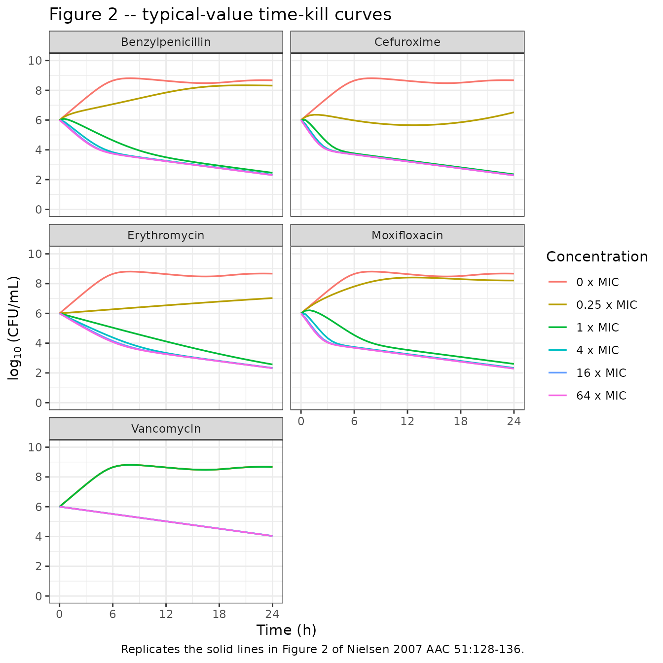
Reproduce the drug-free growth control
Without antibiotics, the model should show exponential growth of the susceptible population from 10^6 CFU/mL up to the stationary-phase carrying capacity Bmax = 4.15e8 CFU/mL (log10 ~ 8.62), with transition of most cells into the resting state at plateau. The paper’s antibiotic-free growth control (Fig 2, top curve in each panel) displays this behaviour.
ev0 <- rxode2::et(amt = 0, cmt = "pen", time = 0) |>
  rxode2::et(seq(0, 48, by = 0.25))
s0  <- rxode2::rxSolve(mod_typ, events = ev0)
s0  <- as.data.frame(s0) |>
  dplyr::mutate(
    total_cfu = bact_susceptible + bact_resting,
    log10_total = log10(pmax(total_cfu, 1)),
    log10_S     = log10(pmax(bact_susceptible, 1)),
    log10_R     = log10(pmax(bact_resting, 1))
  )

ss_reached <- max(s0$log10_total)
target     <- log10(4.15e8)

tibble::tibble(
  quantity = c("Simulated log10(bmax at 48h)", "Paper log10(Bmax)",
               "Fold difference (linear)"),
  value    = c(sprintf("%.3f", ss_reached),
               sprintf("%.3f", target),
               sprintf("%.3fx", 10^(ss_reached - target)))
) |>
  dplyr::rename("Quantity" = quantity, "Value" = value) |>
knitr::kable(caption = "Growth control approaches Bmax at plateau.")| Quantity | Value |
|---|---|
| Simulated log10(bmax at 48h) | 8.810 |
| Paper log10(Bmax) | 8.618 |
| Fold difference (linear) | 1.555x |
s0 |>
  tidyr::pivot_longer(cols = c(log10_total, log10_S, log10_R),
                      names_to = "state", values_to = "log10_cfu") |>
  dplyr::mutate(state = factor(state,
                               levels = c("log10_total", "log10_S", "log10_R"),
                               labels = c("Total S + R", "Susceptible S",
                                          "Resting R"))) |>
  ggplot(aes(time, log10_cfu, colour = state)) +
  geom_line(linewidth = 0.8) +
  geom_hline(yintercept = target, linetype = "dashed", colour = "black") +
  scale_y_continuous(breaks = seq(0, 10, 2), limits = c(0, 10)) +
  labs(
    x = "Time (h)",
    y = expression(log[10]~"(CFU/mL)"),
    colour = "Bacterial state",
    title = "Drug-free growth control: susceptible + resting kinetics",
    caption = "Dashed line: paper Bmax = 4.15e8 CFU/mL (log10 = 8.618)."
  ) +
  theme_bw()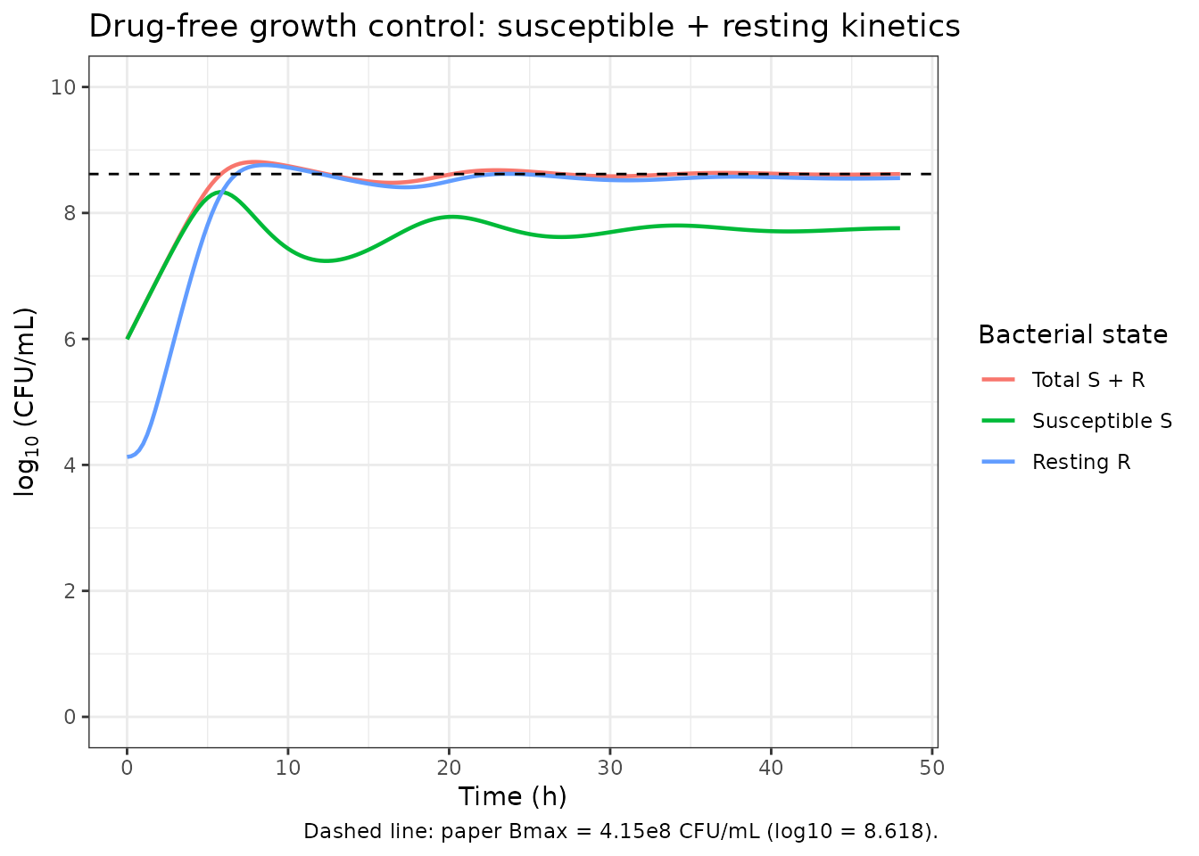
Effect-compartment delay demonstration
Benzylpenicillin, cefuroxime, and moxifloxacin were fit with an estimated biophase equilibration rate constant ke that represents a lag between drug addition and the observed killing (Table 3; Materials and Methods p 129). Erythromycin and vancomycin were fit without a delay (ke fixed to 100 1/h). The biophase state Ce chases the bath concentration C with first-order rate ke; the plot below shows how quickly Ce equilibrates for each drug at 1x MIC.
delay_events <- function(cmt, conc) {
  et <- rxode2::et(amt = conc, cmt = cmt, time = 0) |>
    rxode2::et(seq(0, 12, by = 0.1))
  as.data.frame(et)
}

delay_sim <- purrr::pmap_dfr(
  list(drugs$cmt, drugs$mic_val, drugs$label),
  function(cmt, mic_val, label) {
    ev <- delay_events(cmt, mic_val)
    s  <- rxode2::rxSolve(mod_typ, events = ev)
    df <- as.data.frame(s) |>
      dplyr::mutate(drug = label)
    df$C  <- df[[cmt]]
    df$Ce <- df[[paste0(cmt, "_e")]]
    dplyr::select(df, drug, time, C, Ce)
  }
)

delay_sim |>
  tidyr::pivot_longer(cols = c(C, Ce), names_to = "compartment",
                      values_to = "conc") |>
  ggplot(aes(time, conc, colour = compartment, linetype = compartment)) +
  geom_line(linewidth = 0.7) +
  facet_wrap(~drug, ncol = 2, scales = "free_y") +
  labs(
    x = "Time (h)",
    y = "Concentration (mg/L)",
    colour = "Compartment",
    linetype = "Compartment",
    title = "Effect-compartment delay: C (bath) vs. Ce (biophase) at 1x MIC",
    caption = "PEN / CXM / MXF: estimated ke; ERY / VAN: ke fixed to 100 1/h (near-instant Ce)."
  ) +
  theme_bw()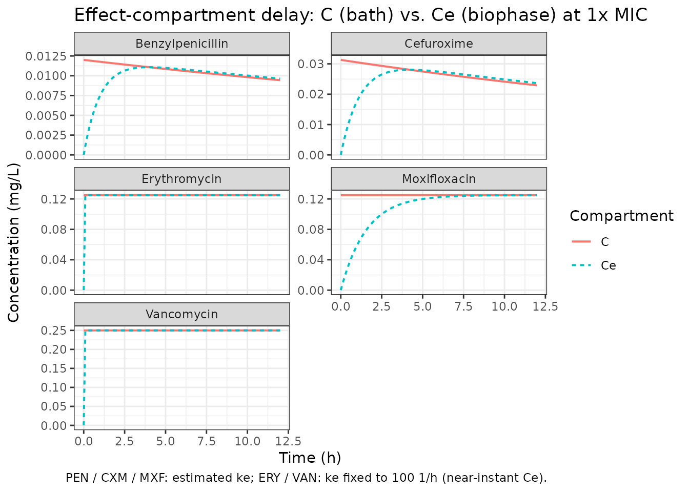
Benzylpenicillin degradation check
Benzylpenicillin and cefuroxime showed significant first-order degradation during the 24-h incubation (Results p 132: kdeg = 0.020 1/h and 0.026 1/h respectively). At the 24 h endpoint, the bath concentration should be exp(-kdeg * 24) of the starting value = exp(-0.020 * 24) = 61.9% for benzylpenicillin and exp(-0.026 * 24) = 53.6% for cefuroxime.
deg_targets <- tibble::tibble(
  drug     = c("Benzylpenicillin", "Cefuroxime"),
  cmt      = c("pen", "cxm"),
  kdeg_1h  = c(0.020, 0.026),
  expected_frac_at_24h = exp(-c(0.020, 0.026) * 24)
)

deg_sim <- purrr::map2_dfr(deg_targets$cmt, deg_targets$drug, function(cmt, label) {
  ev <- rxode2::et(amt = 1, cmt = cmt, time = 0) |>
    rxode2::et(c(0, 24))
  s  <- as.data.frame(rxode2::rxSolve(mod_typ, events = ev))
  s$conc <- s[[cmt]]
  s24 <- s$conc[s$time == 24]
  tibble::tibble(drug = label, sim_frac_at_24h = s24 / 1)
})

deg_check <- deg_targets |>
  dplyr::left_join(deg_sim, by = "drug") |>
  dplyr::mutate(
    pct_diff = abs(sim_frac_at_24h - expected_frac_at_24h) /
      expected_frac_at_24h * 100
  ) |>
  dplyr::select(drug, kdeg_1h, expected_frac_at_24h,
                sim_frac_at_24h, pct_diff)

deg_check |>
  dplyr::rename(
    "Drug"                        = drug,
    "kdeg (1/h)"                  = kdeg_1h,
    "Expected fraction at 24 h"   = expected_frac_at_24h,
    "Simulated fraction at 24 h"  = sim_frac_at_24h,
    "% difference"                = pct_diff
  ) |>
  knitr::kable(digits = 4,
caption = "First-order degradation of PEN and CXM matches the paper's kdeg values.")| Drug | kdeg (1/h) | Expected fraction at 24 h | Simulated fraction at 24 h | % difference |
|---|---|---|---|---|
| Benzylpenicillin | 0.020 | 0.6188 | 0.6188 | 0 |
| Cefuroxime | 0.026 | 0.5358 | 0.5358 | 0 |
Assumptions and deviations
-
Starting inoculum: the paper’s mixture model allocated 74.7% of the 23 starting inocula to mix1 (log-phase, all bacteria in the growing state) and 25.3% to mix2 (approaching stationary, with 5.29% of cells already in the resting state at t = 0). The model file initializes the bacterial compartments at the expected-value marginalization:
bact_susceptible(0) = 10^6 * (1 - fpers_marg)andbact_resting(0) = 10^6 * fpers_margwhere `fpers_marg = (1 - fmix1)- fpers ~
1.3%
. Simulations at low starting inoculum could be overridden viarxSolve(inits = …)` if a true mix1 (all-growing) or mix2 (5.29%-resting) start is required.
- fpers ~
1.3%
Residual error: Nielsen 2007 used the Karlsson 1995 two-component residual model with a replicate-specific SD (47%) and a consistent-across-replicates SD (98%) on natural-log-transformed CFU/mL. For simulation this file collapses the two into a single additive SD on log10(CFU/mL):
addSd = sqrt(0.98^2 + 0.47^2) / log(10) = 0.472. Held FIXED as a simulation-oriented summary of the two-component fit rather than re-estimated.Multi-drug additivity: the DRUG terms sum additively across the five drugs in the model (drug_pen + … + drug_van). In monotherapy, as the paper fitted, only one DRUG term is non-zero at a time. The additive-sum treatment for hypothetical multi-drug simulations is not validated against paper data.
kdeg values for stable drugs: erythromycin, moxifloxacin, and vancomycin were reported as not degrading over 24 h (Results p 132). The model file encodes their
kdegvalues asfixed(log(1e-6))(effectively zero) rather than a strict zero to keep the biophase / drug ODE structure symmetric across drugs and avoid log(0) issues.Between-experiment / between-day variability: the paper reported that estimation of between-experiment or between-day random effects did not improve the fit (Results p 133). No between-experiment variability is encoded here.
Observation floor: the observation
log_cfu = log10(bact_susceptible + bact_resting + 1e-6)includes a small floor to avoid log10(0) if the ODE integrator drives the total to numerical zero at high antibiotic exposure. This does not affect any simulation above the paper’s 10 CFU/mL limit of detection.