Efavirenz (Vujkovic 2018)
Source:vignettes/articles/Vujkovic_2018_efavirenz.Rmd
Vujkovic_2018_efavirenz.RmdModel and source
Citation: Vujkovic M, Bellamy SL, Zuppa AF, Gastonguay MR, Moorthy GS, Ratshaa B, Han X, Steenhoff AP, Mosepele M, Strom BL, Bisson GP, Aplenc R, Gross R (2018). Polymorphisms in cytochrome P450 are associated with extensive efavirenz pharmacokinetics and CNS toxicities in an HIV cohort in Botswana. The Pharmacogenomics Journal 18(5):678-688. doi:10.1038/s41397-018-0028-2. The fixed Vd and Ka values are inherited from the same cohort’s earlier analysis, Gross R et al. (2017) AIDS 31(15):2107-2113, doi:10.1097/QAD.0000000000001593 (paper reference 13).
Description: One-compartment population PK model with first-order absorption for oral efavirenz in HIV-infected black African adults initiating efavirenz-based antiretroviral therapy in Botswana (Vujkovic 2018). Only apparent oral clearance CL/F was estimated: the apparent volume of distribution (150 L) and the absorption rate constant (0.18 /h) were held fixed at the values obtained from the same cohort in the earlier Gross 2017 analysis. CL/F carries a three-level CYP2B6 516G>T (rs3745274) genotype effect (GG 9.439, GT 7.233, TT 4.033 L/h per 70 kg) encoded as log-ratio multiplicative shifts on the 516GG wild-type reference, together with 0.75-exponent allometric scaling of CL/F to a 70 kg reference weight. Residual variability is combined additive plus proportional.
Article: https://doi.org/10.1038/s41397-018-0028-2 (PMC6151142, PMID 29855606)
Vujkovic 2018 is primarily a pharmacogenetic association study. Its
population-pharmacokinetic component is a deliberately minimal
one-compartment model with first-order absorption (NONMEM
ADVAN2, FOCE-I with interaction) in which only
apparent oral clearance CL/F was estimated: the apparent volume
of distribution (150 L) and the absorption rate constant (0.18
h-1) were held fixed at the values obtained from the same
Botswana cohort in the earlier Gross 2017 analysis (paper reference 13).
The single steady-state plasma sample per visit cannot identify volume
or absorption, so this is the appropriate structure for the data - but
it means the model reproduces steady-state exposure far
more reliably than the within-interval concentration-time
shape. The validation below is organised around that
distinction.
Population
The cohort enrolled 941 antiretroviral-naive adults with HIV-1 initiating a first three-drug regimen containing efavirenz 600 mg once daily plus two nucleoside reverse-transcriptase inhibitors, at clinics in and around Gaborone, Botswana, between June 2009 and November 2013. Inclusion required confirmed HIV infection, black African origin, no pregnancy or pregnancy intention, and age 21 years or older. 814 participants were successfully genotyped for CYP2B6 516G>T (rs3745274) and 742 of those contributed at least one steady-state plasma efavirenz concentration at month 1; 562 also contributed a month-6 sample.
Baseline characteristics (Vujkovic 2018 Table 1): median age 37 years (IQR 33-44), 49.0% male, median body mass index 22.0 kg/m2 (IQR 19.8-25.1), median CD4 count 196 cells/mm3 (IQR 112-256), median plasma viral load 4.9 log10 copies/mL (IQR 4.2-5.4), history of tuberculosis in 3.8%. Median observed plasma efavirenz was 2.17 ug/mL (IQR 1.62-3.88) at month 1 and 2.05 ug/mL at month 6.
Table 1 reports body mass index but neither body weight nor height, so the cohort weight distribution is not recoverable from the paper. Every simulation below is therefore run at the model’s own allometric reference weight of 70 kg, where the weight factor is exactly 1 and the published typical clearances apply directly. See Assumptions and deviations.
The same information is available programmatically via
readModelDb("Vujkovic_2018_efavirenz")()$population.
Source trace
Every ini() entry in
inst/modeldb/specificDrugs/Vujkovic_2018_efavirenz.R
carries an in-file comment naming its origin. They are collected here
for review.
| Equation / parameter | Value | Source location |
|---|---|---|
lcl (CL/F, 516GG reference) |
log(9.439) L/h per 70 kg |
Results Population Pharmacokinetics para. 1: “normal (GG, 9.439 L/hr/70kg)” |
e_516gt_cl |
log(7.233 / 9.439) = -0.2662 |
Results Population Pharmacokinetics para. 1: “slow (GT, 7.233 L/hr/70kg)” |
e_516tt_cl |
log(4.033 / 9.439) = -0.8503 |
Results Population Pharmacokinetics para. 1: “very slow (TT, 4.033 L/hr/70kg)” |
lvc (Vd/F) |
fixed(log(150)) L |
Methods Population PK Model Development para. 1: “holding the parameters of volume of distribution (Vd) and absorption rate constant (Ka) constant at 150 L and 0.18 h-1 respectively [13]” |
lka |
fixed(log(0.18)) 1/h |
Methods Population PK Model Development para. 1, same sentence |
e_wt_cl |
fixed(0.75) |
Methods Population PK Model Development para. 2: “Weight was included in an allometric model and fixed at 0.75 CL/F and normalized to a reference weight of 70 kg” |
etalcl |
0.15189 = log(1 + 0.405^2)
|
Results Population Pharmacokinetics para. 1: “inter-individual variability (omega2 CL) of 40.5% coefficient variation” |
propSd |
0.0831 |
Results Population Pharmacokinetics para. 1: “proportional residual variability of 0.0831” |
addSd |
0.0699 mg/L |
Results Population Pharmacokinetics para. 1: “residual additive variability of 0.0699 SD” |
d/dt(depot), d/dt(central)
|
n/a | Methods Population PK Model Development para. 1: “The ADVAN2 subroutine (one compartment linear model with first order absorption) was selected” |
| Combined additive + proportional error | n/a | Methods Population PK Model Development para. 2: “A composite additive and proportional error model was used” |
| Genotype counts used for the mixture cohort | GG 309 / GT 375 / TT 115 | Table 3, summed over the 983T>C and extensive-SNP strata |
| Observed concentration distribution | median 2.17 (IQR 1.62-3.88) ug/mL | Results Population Pharmacokinetics para. 1 and Table 1 |
Virtual cohorts
Original observed data are not publicly available. Two cohorts are used:
- A typical-value cohort of five subjects with the random effects zeroed: the three CYP2B6 516G>T genotypes at the 70 kg allometric reference, plus two extra 516GG subjects at 50 kg and 90 kg to exercise the allometric term. This cohort supports the deterministic checks (clearance recovery, exposure ratios, allometric exponent), where the only error is trapezoidal.
- A stochastic mixture cohort of 200 subjects whose genotypes are drawn in the proportions implied by Vujkovic 2018 Table 3 (GG 39%, GT 47%, TT 14%), carrying between-subject variability on CL/F and the combined residual error. This cohort is compared against the observed concentration distribution in Table 1.
set.seed() seeds R’s RNG only. rxode2’s simulation RNG
is partitioned per solver thread, so the stochastic cohort differs
between a 2-core CI runner and a 16-thread workstation and no seed makes
them agree. Every assertion on a cohort-derived quantity below is
written to hold for any cohort the model can produce; the deterministic
assertions are separately tight because they have no cohort in them at
all.
set.seed(20180601)

tau    <- 24     # dosing interval (h)
n_dose <- 21     # days of once-daily dosing; efavirenz reaches steady state in 6-10 days
t_last <- (n_dose - 1) * tau   # time of the final dose (h)

# One subject's event table: n_dose daily 600 mg oral doses into `depot`, then
# observations across the final dosing interval on the `central` ODE state.
# `cmt` on the observation rows names an ODE STATE, never the algebraic
# observable `Cc`.
make_subjects <- function(ids, snp, wt, grid) {
  stopifnot(length(ids) == length(snp), length(ids) == length(wt))
  key <- tibble(id = ids, SNP_CYP2B6_RS3745274_T_COUNT = snp, WT = wt)
  doses <- key |>
    tidyr::expand_grid(time = seq(0, by = tau, length.out = n_dose)) |>
    mutate(amt = 600, evid = 1L, cmt = "depot")
  obs <- key |>
    tidyr::expand_grid(time = t_last + grid) |>
    mutate(amt = NA_real_, evid = 0L, cmt = "central")
  bind_rows(doses, obs) |>
    arrange(id, time, desc(evid))
}

geno_label <- c("516GG", "516GT", "516TT")

# --- cohort 1: typical values -------------------------------------------------
ev_typ <- make_subjects(
  ids  = 1:5,
  snp  = c(0L, 1L, 2L, 0L, 0L),
  wt   = c(70, 70, 70, 50, 90),
  grid = seq(0, tau, by = 0.1)      # fine grid: trapezoidal AUC error is negligible
) |>
  mutate(
    genotype = geno_label[SNP_CYP2B6_RS3745274_T_COUNT + 1L],
    arm      = paste0(genotype, ", ", WT, " kg")
  )

# --- cohort 2: stochastic genotype mixture ------------------------------------
n_mix     <- 200                       # <= 200 per arm (single arm here)
geno_n    <- c(GG = 309, GT = 375, TT = 115)   # Vujkovic 2018 Table 3
geno_prob <- geno_n / sum(geno_n)

ev_mix <- make_subjects(
  ids  = 1000L + seq_len(n_mix),                       # disjoint from cohort 1
  snp  = sample(c(0L, 1L, 2L), n_mix, replace = TRUE, prob = geno_prob),
  wt   = rep(70, n_mix),
  grid = seq(0, tau, by = 0.5)
) |>
  mutate(genotype = geno_label[SNP_CYP2B6_RS3745274_T_COUNT + 1L], arm = "mixture")

events <- bind_rows(ev_typ, ev_mix)
stopifnot(!anyDuplicated(unique(events[, c("id", "time", "evid")])))
Simulation
mod <- readModelDb("Vujkovic_2018_efavirenz")

# Deterministic: random effects zeroed, so `Cc` is the typical-value prediction.
sim_typ <- rxode2::rxSolve(
  rxode2::zeroRe(mod),
  events = ev_typ,
  keep   = c("genotype", "arm", "WT")
) |>
  as.data.frame() |>
  filter(!is.na(Cc))
#> ℹ omega/sigma items treated as zero: 'etalcl'
#> Warning: multi-subject simulation without without 'omega'

# Stochastic: `Cc` is the individual prediction, `sim` adds the combined
# additive + proportional residual error and is therefore the column that
# corresponds to a MEASURED concentration.
sim_mix <- rxode2::rxSolve(
  mod,
  events = ev_mix,
  keep   = c("genotype", "arm", "WT")
) |>
  as.data.frame() |>
  filter(!is.na(Cc))

cat("typical rows:", nrow(sim_typ), " mixture rows:", nrow(sim_mix), "\n")
#> typical rows: 1205  mixture rows: 9800
stopifnot(nrow(sim_typ) > 0, nrow(sim_mix) > 0, all(c("Cc", "sim") %in% names(sim_mix)))
Steady-state profiles by CYP2B6 516G>T genotype
The paper publishes no concentration-time figure (Figure 1 is a linkage- disequilibrium map and Figure 2 is a CNS-toxicity boxplot by composite metaboliser group), so there is no PK figure to replicate. The panel below instead makes the model’s genotype separation visible, which is what Table 2 and the Results paragraph quantify.
sim_typ |>
  filter(WT == 70) |>
  mutate(tad = time - t_last) |>
  ggplot(aes(tad, Cc, colour = genotype)) +
  geom_line(linewidth = 0.9) +
  labs(
    x = "Time after the final dose (h)",
    y = "Efavirenz plasma concentration (mg/L)",
    colour = "CYP2B6 516G>T",
    title = "Typical steady-state profiles, efavirenz 600 mg once daily at 70 kg",
    caption = "Quantifies the genotype effect reported in Vujkovic 2018 Results / Table 2."
  ) +
  theme_bw()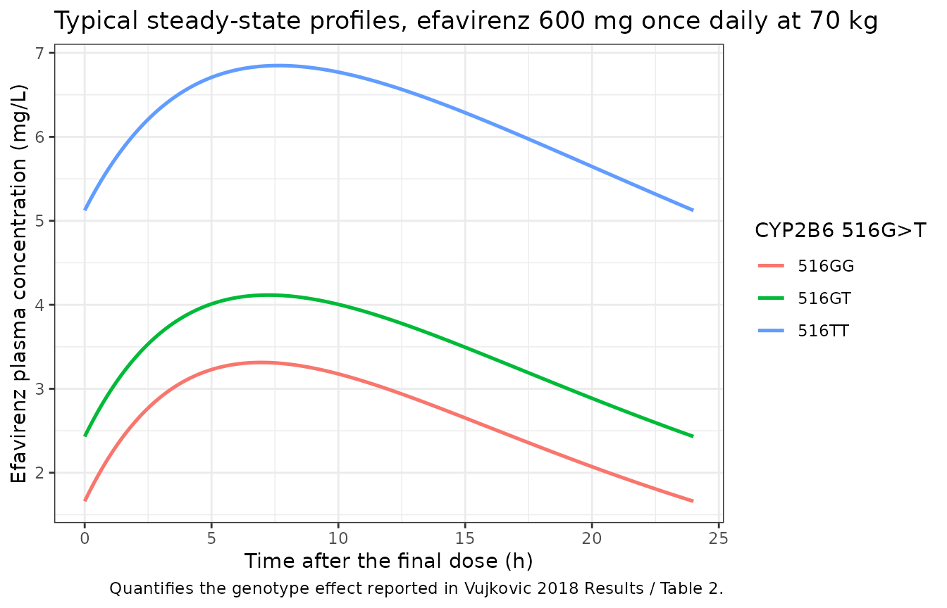
sim_mix |>
  mutate(tad = time - t_last) |>
  group_by(tad, genotype) |>
  summarise(
    Q05 = quantile(sim, 0.05), Q50 = quantile(sim, 0.50),
    Q95 = quantile(sim, 0.95), n = dplyr::n(), .groups = "drop"
  ) |>
  ggplot(aes(tad, Q50)) +
  geom_ribbon(aes(ymin = Q05, ymax = Q95), alpha = 0.25) +
  geom_line() +
  facet_wrap(~genotype) +
  labs(
    x = "Time after the final dose (h)",
    y = "Efavirenz plasma concentration (mg/L)",
    title = "Simulated steady-state spread in the 200-subject mixture cohort",
    caption = "Median with 5th-95th percentile band, residual error included."
  ) +
  theme_bw()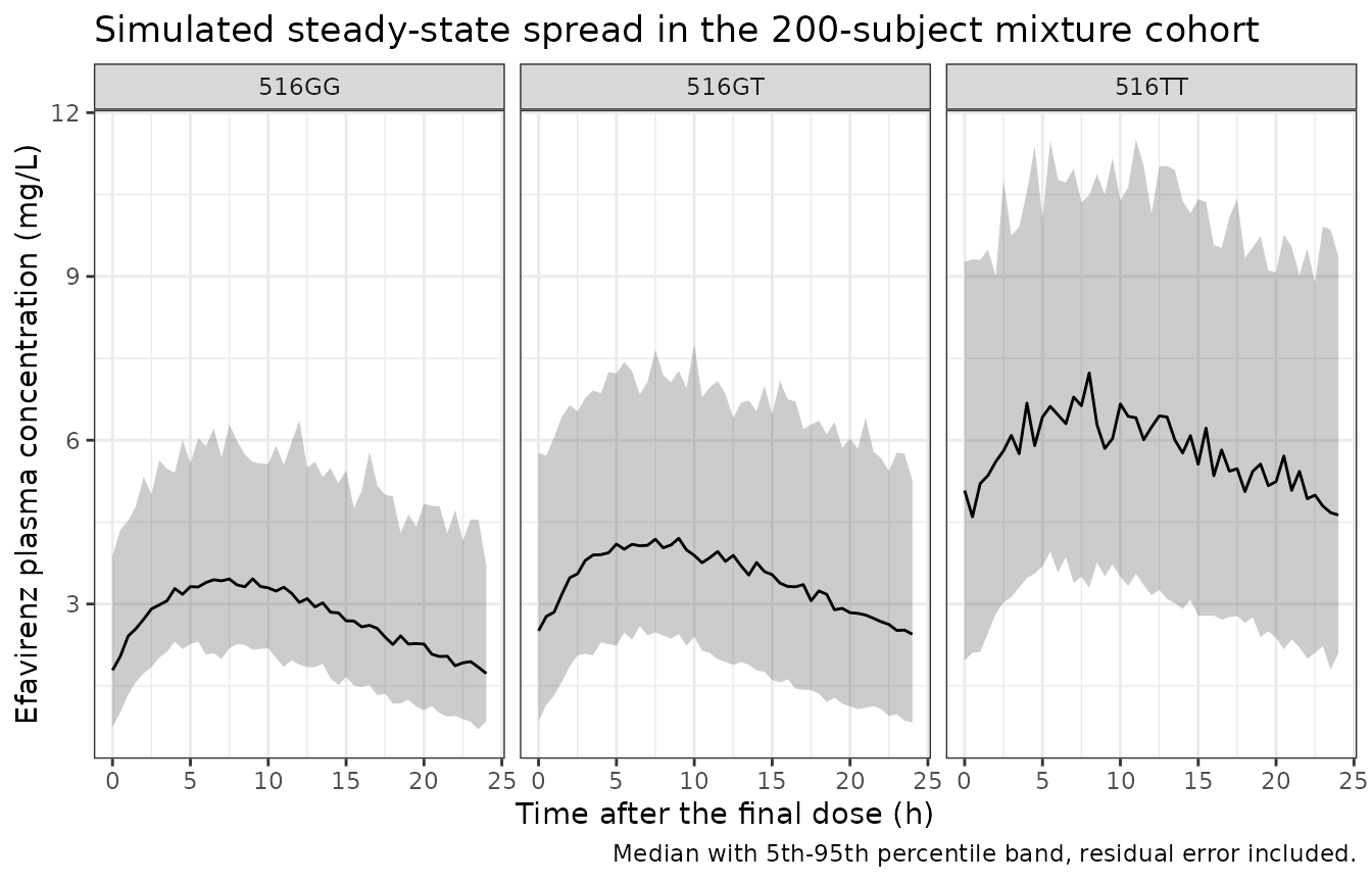
PKNCA validation
Steady-state NCA over the final dosing interval, on the typical-value
cohort. Grouping is by arm (genotype x weight) so each
published typical clearance gets its own row.
sim_nca <- sim_typ |>
  filter(!is.na(Cc)) |>
  select(id, time, Cc, arm)

# Guarantee a record at the interval start for every subject. Here the
# interval starts at the final dose, t_last, which the 0.1 h grid already
# contains; the bind_rows keeps the guarantee explicit and idempotent.
sim_nca <- bind_rows(
  sim_nca,
  sim_nca |> distinct(id, arm) |> mutate(time = t_last, Cc = 0)
) |>
  distinct(id, arm, time, .keep_all = TRUE) |>
  arrange(id, arm, time)

dose_df <- ev_typ |>
  filter(evid == 1L, time == t_last) |>
  select(id, time, amt, arm)

conc_obj <- PKNCA::PKNCAconc(sim_nca, Cc ~ time | arm + id,
                             concu = "mg/L", timeu = "h")
dose_obj <- PKNCA::PKNCAdose(dose_df, amt ~ time | arm + id, doseu = "mg")

intervals <- data.frame(
  start   = t_last,
  end     = t_last + tau,
  cmax    = TRUE,
  tmax    = TRUE,
  cmin    = TRUE,
  clast.obs = TRUE,
  cav     = TRUE,
  auclast = TRUE,
  cl.last = TRUE
)

nca_res <- PKNCA::pk.nca(PKNCA::PKNCAdata(conc_obj, dose_obj, intervals = intervals))

nca_wide <- as.data.frame(nca_res$result) |>
  select(arm, PPTESTCD, PPORRES) |>
  tidyr::pivot_wider(names_from = PPTESTCD, values_from = PPORRES)

nca_wide |>
  rename(
    "Arm"                    = arm,
    "Cmax (mg/L)"            = cmax,
    "Tmax (h)"               = tmax,
    "Cmin (mg/L)"            = cmin,
    "Clast (mg/L)"           = clast.obs,
    "Cav (mg/L)"             = cav,
    "AUC0-tau (mg*h/L)"      = auclast,
    "CL/F (L/h)"             = cl.last
  ) |>
knitr::kable(digits = 3, caption = "Steady-state NCA of the typical-value profiles.")| Arm | AUC0-tau (mg*h/L) | Cmax (mg/L) | Cmin (mg/L) | Tmax (h) | Clast (mg/L) | CL/F (L/h) | Cav (mg/L) |
|---|---|---|---|---|---|---|---|
| 516GG, 50 kg | 81.812 | 4.069 | 2.385 | 7.2 | 2.385 | 7.334 | 3.409 |
| 516GG, 70 kg | 63.565 | 3.313 | 1.660 | 7.0 | 1.660 | 9.439 | 2.649 |
| 516GG, 90 kg | 52.646 | 2.861 | 1.239 | 6.7 | 1.239 | 11.397 | 2.194 |
| 516GT, 70 kg | 82.952 | 4.116 | 2.431 | 7.2 | 2.431 | 7.233 | 3.456 |
| 516TT, 70 kg | 148.772 | 6.848 | 5.124 | 7.6 | 5.124 | 4.033 | 6.199 |
Comparison against the published clearances
The paper reports the three genotype-specific typical apparent
clearances at 70 kg. Recovering them as dose / AUC0-tau
from the solved model is a closed-form check on the encoding: same
parameters on both sides, so the only discrepancy possible is
trapezoidal integration error.
published <- tibble::tribble(
  ~arm,             ~cl.last,
  "516GG, 70 kg",   9.439,
  "516GT, 70 kg",   7.233,
  "516TT, 70 kg",   4.033
)

cmp <- nlmixr2lib::ncaComparisonTable(
  simulated     = nca_res,
  reference     = published,
  by            = "arm",
  units         = c(cl.last = "L/h"),
  tolerance_pct = 20
)
#> Warning: ncaParamLabel(): unknown PKNCA code(s) returned as-is: 'cl.last'

knitr::kable(
  cmp,
  caption = "Simulated vs. published typical CL/F. * differs from reference by >20%.",
  align   = c("l", "l", "r", "r", "r")
)| NCA parameter | arm | Reference | Simulated | % diff |
|---|---|---|---|---|
| cl.last (L/h) | 516GG, 70 kg | 9.44 | 9.44 | +0.0% |
| cl.last (L/h) | 516GT, 70 kg | 7.23 | 7.23 | +0.0% |
| cl.last (L/h) | 516TT, 70 kg | 4.03 | 4.03 | +0.0% |
cl_sim <- nca_wide |>
  filter(arm %in% published$arm) |>
  select(arm, cl_sim = cl.last) |>
  left_join(published |> rename(cl_pub = cl.last), by = "arm") |>
  mutate(pct = 100 * (cl_sim - cl_pub) / cl_pub)

knitr::kable(cl_sim, digits = 4,
caption = "Clearance recovery, per cent difference from the published value.")| arm | cl_sim | cl_pub | pct |
|---|---|---|---|
| 516GG, 70 kg | 9.4391 | 9.439 | 1e-03 |
| 516GT, 70 kg | 7.2331 | 7.233 | 8e-04 |
| 516TT, 70 kg | 4.0330 | 4.033 | 6e-04 |
Genotype exposure ratios
auc <- setNames(nca_wide$auclast, nca_wide$arm)

ratio_tab <- tibble(
  comparison = c("516GG / 516GT", "516GG / 516TT"),
  simulated  = c(auc[["516GT, 70 kg"]] / auc[["516GG, 70 kg"]],
                 auc[["516TT, 70 kg"]] / auc[["516GG, 70 kg"]]),
  published  = c(9.439 / 7.233, 9.439 / 4.033)
) |>
  mutate(pct = 100 * (simulated - published) / published)

knitr::kable(ratio_tab, digits = 4,
caption = "Steady-state AUC ratio vs the inverse published clearance ratio.")| comparison | simulated | published | pct |
|---|---|---|---|
| 516GG / 516GT | 1.3050 | 1.3050 | 3e-04 |
| 516GG / 516TT | 2.3405 | 2.3404 | 5e-04 |
Allometric exponent
The 50 kg and 90 kg 516GG arms recover the fixed 0.75 exponent exactly, since clearance is the only weight-scaled parameter.
allo <- nca_wide |>
  filter(grepl("^516GG", arm)) |>
  mutate(WT = as.numeric(sub(".*, ", "", sub(" kg$", "", arm)))) |>
  transmute(WT, cl = cl.last,
            ratio_sim = cl / cl[WT == 70],
            ratio_exp = (WT / 70)^0.75,
            pct = 100 * (ratio_sim - ratio_exp) / ratio_exp)

knitr::kable(allo, digits = 4,
caption = "CL/F vs body weight for the 516GG genotype.")| WT | cl | ratio_sim | ratio_exp | pct |
|---|---|---|---|---|
| 50 | 7.3339 | 0.7770 | 0.7770 | -2e-04 |
| 70 | 9.4391 | 1.0000 | 1.0000 | 0e+00 |
| 90 | 11.3970 | 1.2074 | 1.2074 | 2e-04 |
Genotype-weighted clearance vs the paper’s covariate-free base model
Before the genotype term was added, the paper’s base model gave a typical clearance of 7.3 L/h per 70 kg at month 1 and 7.6 L/h per 70 kg at month 6. Averaging the three published genotype-specific clearances over the genotype counts in Table 3 - two different parts of the paper - must land in that neighbourhood. This is an independent falsifier of the transcription: it uses Table 3, which was not used to build the model.
cl_pub <- c(GG = 9.439, GT = 7.233, TT = 4.033)
cl_weighted <- sum(geno_prob * cl_pub)

cat(sprintf("Genotype-weighted typical CL/F: %.3f L/h per 70 kg\n", cl_weighted))
#> Genotype-weighted typical CL/F: 7.626 L/h per 70 kg
cat("Paper's covariate-free base model:  7.3 (month 1) and 7.6 (month 6) L/h per 70 kg\n")
#> Paper's covariate-free base model:  7.3 (month 1) and 7.6 (month 6) L/h per 70 kg

# Deterministic (published numbers only, no simulation). Bracket the two
# base-model values the paper prints, with headroom for the rounding they
# were reported to.
stopifnot(cl_weighted > 7.0, cl_weighted < 8.0)
Observed concentration distribution (Table 1)
The paper reports a median observed plasma efavirenz of 2.17 ug/mL
(IQR 1.62-3.88) at month 1, from single steady-state draws whose time
after dose was recorded but is not published. Two comparisons are made
against the 200-subject mixture cohort, using the sim
column (individual prediction plus the combined residual error), which
is what a measured sample corresponds to:
- against the concentration distribution pooled over the whole dosing interval, which brackets every possible sampling time; and
- against the end-of-interval (24 h post-dose) distribution.
pub_med <- 2.17
pub_iqr <- c(1.62, 3.88)

interval_q <- quantile(sim_mix$sim, c(0.10, 0.25, 0.50, 0.75, 0.90))
trough <- sim_mix |> filter(abs(time - (t_last + tau)) < 1e-6)
trough_q <- quantile(trough$sim, c(0.10, 0.25, 0.50, 0.75, 0.90))

obs_tab <- tibble(
  Source = c("Vujkovic 2018 Table 1 (observed, month 1)",
             "Simulated, pooled over the dosing interval",
             "Simulated, 24 h after the dose"),
  `10th %ile` = c(NA, interval_q[["10%"]], trough_q[["10%"]]),
  `25th %ile` = c(pub_iqr[1], interval_q[["25%"]], trough_q[["25%"]]),
  Median      = c(pub_med, interval_q[["50%"]], trough_q[["50%"]]),
  `75th %ile` = c(pub_iqr[2], interval_q[["75%"]], trough_q[["75%"]]),
  `90th %ile` = c(NA, interval_q[["90%"]], trough_q[["90%"]])
)

knitr::kable(obs_tab, digits = 3,
caption = "Observed vs simulated steady-state concentrations (mg/L = ug/mL).")| Source | 10th %ile | 25th %ile | Median | 75th %ile | 90th %ile |
|---|---|---|---|---|---|
| Vujkovic 2018 Table 1 (observed, month 1) | NA | 1.620 | 2.170 | 3.880 | NA |
| Simulated, pooled over the dosing interval | 1.741 | 2.430 | 3.337 | 4.597 | 6.404 |
| Simulated, 24 h after the dose | 1.063 | 1.543 | 2.331 | 3.292 | 5.197 |
trough_pct <- 100 * (trough_q[["50%"]] - pub_med) / pub_med
cat(sprintf("End-of-interval median differs from the published median by %.1f%%\n",
            trough_pct))
#> End-of-interval median differs from the published median by 7.4%

# Cohort-derived, so both bounds are robust rather than tight. Measured at
# 1 / 2 / 3 / 4 / 8 / 16 solver threads (identical on all six here, because the
# eta draw for this cohort turned out not to be partitioned across threads) and
# on three independently-drawn genotype mixtures obtained by varying the RNG
# consumption ahead of the solve. Those alternative draws are the relevant
# spread, not the thread count.
#
# (a) The published median must sit inside the simulated interval-wide 10th-90th
#     percentile band. Realised bands across the draws: 1.74-6.40, 1.61-6.86,
#     1.66-6.25, 1.49-6.80. 2.17 sits inside all of them, with at least 25%
#     margin to the lower edge. A dose, volume or clearance mis-transcription of
#     ~1.3x or more moves the band off the published value.
stopifnot(pub_med > interval_q[["10%"]], pub_med < interval_q[["90%"]])

# (b) The end-of-interval median tracks the published median closely. Realised
#     across the same draws: +7.4%, +7.1%, +2.8%, -2.3%. 25% leaves that spread
#     roughly 3x of headroom while still going red on a clearance or dose error
#     of a few tens of per cent - the errors this check exists to catch.
stopifnot(abs(trough_pct) < 25)
The agreement at the end of the dosing interval is close, and the published median sits comfortably inside the interval-wide simulated band. This is the expected shape of the result: CL/F is the only quantity the paper estimated, so steady-state exposure is well reproduced, while where within the interval a given concentration falls depends on the inherited Vd/F and ka, which were fixed rather than fitted (see Assumptions and deviations).
Assumptions and deviations
-
Body weight is not reported. Vujkovic 2018 Table 1 gives body mass index (median 22.0 kg/m2, IQR 19.8-25.1) but neither weight nor height, so no cohort weight distribution can be reconstructed. All simulations here run at the model’s own 70 kg allometric reference, where the weight factor is exactly
- Downstream users supplying real weights get the published clearances
scaled by
(WT/70)^0.75.
- Downstream users supplying real weights get the published clearances
scaled by
Inter-occasion variability is not encoded. The final model retained inter-occasion variability on CL/F between the month-1 and month-6 visits (Table 2 footnote: “Clearance estimates are corrected for the covariates: CYP2B6 G516T genotype (rs3745274), allometrically scaled weight, and inter-occasional variability between visits”), but its magnitude is never reported for the final model. The only quantification anywhere in the paper is from the pre-genotype base model - “3% higher apparent clearance at month 6 compared to month 1 measurements (7.3 vs. 7.6 L/hr/70kg)” - which belongs to a different model and is not carried here. Omitting an unreported variance term follows the convention already used in
Bienczak_2016_efavirenzandSvensson_2018_bedaquilinewhen a between-subject term is reported on the same parameter. The consequence is that this model has no occasion-to-occasion component; between-subject variability (40.5% CV) is unaffected.Variability numbers are read on the SD scale. The Results paragraph reports “inter-individual variability (omega2 CL) of 40.5% coefficient variation, proportional residual variability of 0.0831% coefficient variation, and residual additive variability of 0.0699 SD”. The stated unit is taken over the omega-squared symbol throughout: 40.5% is read as a CV and converted to the log-scale variance
log(1 + 0.405^2) = 0.15189, 0.0831 as a proportional SD (8.31% CV), and 0.0699 as an additive SD in mg/L. Reading 0.0831 as a variance instead would give a proportional SD of 0.288 (28.8%); the paper’s own wording (“SD” for the additive term, “coefficient variation” for the proportional one) supports the SD reading, and the choice affects only the width of the residual band, not any structural parameter or the exposure comparisons above.Vd/F and ka are inherited, not fitted. Both were fixed from Gross 2017 (AIDS 31(15):2107-2113, paper reference 13) on the same cohort, which the present paper states explicitly. The resulting elimination half-life (
log(2) * 150 / CL, about 11 h at the 516GG typical clearance) is much shorter than efavirenz’s true terminal half-life of 40-55 h, because a single midpoint sample per visit cannot identify a distribution phase. Use this model for steady-state exposure, genotype stratification and dose-proportionality work; do not use it to predict the shape of a rich single-dose profile.The 983T>C effect is documented but not carried. CYP2B6 983T>C (rs28399499) had the strongest univariate signal in Table 2 (7.984 / 4.691 / 1.440 L/h per 70 kg by genotype, MOFV 1862 versus 2075 for the pre-SNP model), but the paper did not build a joint multivariate PK model containing both it and 516G>T - it used the pair, plus the extensive-metaboliser alleles, to define the composite metaboliser group of Table 3 for the pharmacodynamic analyses. Carrying the univariate 983T>C estimate alongside the retained 516G>T effect would double-count the shared CYP2B6 signal, so it is recorded in
covariatesDataExcludedrather than incovariateData. The same applies to the other 20 screened SNPs in Table 2, and to sex, tuberculosis history and adherence, which were tested and not retained.The pharmacodynamic analyses are out of scope. The paper’s CNS-toxicity and treatment-outcome analyses are a proportional-odds ordinal regression and logistic regressions of clinical endpoints on the composite CYP2B6 metaboliser group (Figure 2, Table 4). They are association models on a genotype grouping, not exposure-response models - no efavirenz concentration or exposure metric enters them - so they have no structural pharmacometric form to encode and are not part of this extraction.
No published PK figure or NCA table exists to replicate. The paper reports no concentration-time figure and no NCA parameters. The validation above therefore uses what the paper does publish: the three genotype-specific typical clearances, the covariate-free base-model clearance, the genotype counts in Table 3, and the observed concentration distribution in Table 1.