Remlifanserin (Darwish 2026)
Source:vignettes/articles/Darwish_2026_remlifanserin.Rmd
Darwish_2026_remlifanserin.RmdModel and source
- Citation: Darwish M, Lin N, Dirks B, Jaworowicz D, Maxwell K, Pathak S. Population pharmacokinetics of remlifanserin (ACP-204), a serotonin 2A receptor inverse agonist. Alzheimer’s & Dementia: Translational Research & Clinical Interventions. 2026;12(1):e70254. doi:10.1002/trc2.70254
- Description: Population PK model for oral remlifanserin (ACP-204), a selective 5-HT2A receptor inverse agonist (Darwish 2026): one-compartment with first-order absorption, an absorption lag time and linear elimination, pooled across seven Phase 1 studies in healthy young and older adults. Fed status shifts the absorption lag time and female sex lowers the apparent central volume.
- Article: https://doi.org/10.1002/trc2.70254
- Supplement (Supplemental Tables 1-6 and the NONMEM control stream): https://europepmc.org/article/PMC/PMC13133547
Remlifanserin (ACP-204) is a selective serotonin 2A (5-HT2A) receptor inverse agonist in development for Alzheimer’s disease psychosis and Lewy body dementia psychosis. Darwish 2026 is the first population PK model for the compound.
Units
The model is parameterised in days, exactly as
Darwish 2026 Table 1 and the Supplemental Methods control stream report
it. The control stream’s scaling line reads
S2=V ;Dose amount = ug; Volume = L; Concentration = ng/mL,
so dose amounts are entered in micrograms: the 60 mg
target dose is 60000. Darwish 2026 Section 3.4 restates the
identical estimates in hours (CL/F 35.4 L/h, Ka 0.692 1/h,
ALAG1 0.720 h fasted); those are conversions of the same numbers, not a
separate parameterisation.
Population
The model was fit to 3935 plasma concentrations from 209 healthy
participants pooled across seven Phase 1 studies of remlifanserin
(Supplemental Table 1): a single-ascending-dose study with a food arm
(001), a multiple-ascending-dose study that included an elderly cohort
(002), a PET receptor-occupancy study (003), itraconazole and
carbamazepine drug-drug-interaction studies (004 and 005, of which only
period 1 was retained), a crossover food-effect study (010), and a
[14C] mass-balance study (011). Oral doses spanned 10 to
180 mg, given as single doses and as once-daily multiple doses for 10
days.
Participants were 19 to 75 years old (median 37), weighed 47 to 108 kg (median 77.6), and had a BMI of 18.5 to 31.9 kg/m2 (median 26.3). 30.6% (64/209) were female. Race was 59.3% White, 33.0% Black or African American, 2.87% Asian and 4.78% Other. Renal and hepatic function were predominantly normal (eGFR 58.4 to 138 mL/min/1.73 m2, median 103). Only 18 participants were in the 65-75 year older-adult stratum, which Darwish 2026 Section 4.3 flags as a limitation. Baseline demographics are Supplemental Table 2; the fed/fasted record split (71% fasted, 29% fed) is Supplemental Table 3.
The same information is available programmatically via
readModelDb("Darwish_2026_remlifanserin")()$population.
Source trace
The per-parameter origin is recorded as an in-file comment next to
each ini() entry in
inst/modeldb/specificDrugs/Darwish_2026_remlifanserin.R.
The table below collects them in one place for review.
| Equation / parameter | Value | Source location |
|---|---|---|
| Structural model: 1-compartment, first-order absorption, absorption lag, linear elimination | n/a | Section 3.1; Supplemental Methods
$SUBROUTINES ADVAN2 TRANS2
|
lcl (CL/F) |
log(849) L/day |
Table 1, “CL/F (L/day)” = 849, RSE 2.84% |
lvc (V/F, male) |
log(930) L |
Table 1, “V/F (L)” = 930, RSE 2.43% |
lka (Ka) |
log(16.6) 1/day |
Table 1, “Ka (1/day)” = 16.6, RSE 4.65% |
ltlag (ALAG1, fasted) |
log(0.0300) day |
Table 1, “ALAG1 (day)” = 0.0300, RSE 1.91% |
e_sexf_vc |
-131 L | Table 1, “Additive shift in V/F for females” = -131, RSE 16.8% |
e_fed_tlag |
0.290 | Table 1, “Proportional shift in ALAG1 for fed status” = 0.290, RSE 10.4% |
vc <- (exp(lvc) + e_sexf_vc * SEXF) * exp(etalvc) |
n/a | Section 3.2 equation V/F_i = 930 L - 131 * female_i;
$PK block TVV = TVVI + COV2,
V = TVV*EXP(ETA(2))
|
tlag <- exp(ltlag) * (1 + e_fed_tlag * FED) * exp(etaltlag) |
n/a | Section 3.2 equation
ALAG1_i = 0.0300 d * (1 + 0.290 * fed_i); $PK
block TVALAG1 = THETA(4)*(1+THETA(5)*FED)
|
etalcl variance |
0.1668 | Table 1, CL/F 42.6 %CV, back-transformed as
log(1 + 0.426^2)
|
etalvc variance |
0.0981 | Table 1, V/F 32.1 %CV, back-transformed as
log(1 + 0.321^2)
|
etalcl-etalvc covariance |
0.109 | Table 1, “Covariance (IIV in V/F, IIV in CL/F)” = 0.109, RSE 11.9% |
etalka variance |
0.3754 | Table 1, Ka 67.5 %CV, back-transformed as
log(1 + 0.675^2)
|
etaltlag variance |
0.01138 | Table 1, ALAG1 10.7 %CV, back-transformed as
log(1 + 0.107^2)
|
propSd |
0.197 | Table 1, “Residual variability” = 0.0388 (a variance), reported as
19.7 %CV; sqrt(0.0388) = 0.1970 |
Pinning the omega scale
Darwish 2026 prints interindividual variability only as a percent CV,
so each variance had to be back-transformed. Two independent checks
establish that the paper used the log-normal relation
omega^2 = log(1 + CV^2) rather than the
omega = CV approximation.
cv <- c(cl = 0.426, vc = 0.321)            # Table 1, %CV column
covariance <- 0.109                         # Table 1, covariance row

omega2_lognormal <- log(1 + cv^2)           # candidate A
omega2_cvdirect  <- cv^2                    # candidate B

r_lognormal <- covariance / sqrt(prod(omega2_lognormal))
r_cvdirect  <- covariance / sqrt(prod(omega2_cvdirect))

# Table 1 footnote: "The calculated correlation coefficient (r) associated with
# covariance (IIV in V/F, IIV in CL/F) was 0.852 with r^2 = 0.726."
data.frame(
  scale = c("omega^2 = log(1 + CV^2)", "omega^2 = CV^2"),
  r     = c(r_lognormal, r_cvdirect),
  r2    = c(r_lognormal, r_cvdirect)^2,
  published_r = 0.852,
  published_r2 = 0.726
) |>
knitr::kable(digits = 4, caption = "Which omega scale reproduces the Table 1 footnote?")| scale | r | r2 | published_r | published_r2 |
|---|---|---|---|---|
| omega^2 = log(1 + CV^2) | 0.8523 | 0.7265 | 0.852 | 0.726 |
| omega^2 = CV^2 | 0.7971 | 0.6354 | 0.852 | 0.726 |
# The log-normal back-transform reproduces the published r to three decimals;
# the CV-squared alternative is off by more than 0.05. Gate on the footnote.
stopifnot(
  abs(r_lognormal - 0.852) < 0.002,
  abs(r_lognormal^2 - 0.726) < 0.002,
  abs(r_cvdirect - 0.852) > 0.02
)
The Supplemental Methods $OMEGA initial estimates (0.16
for CL/F, 0.09 for V/F, 0.10 for the covariance, 0.30 for Ka,
0.01 for ALAG1) sit next to the back-transformed final values (0.1668,
0.0981, 0.109, 0.3754, 0.01138), independently confirming that these are
NONMEM variances on the log scale.
Typical-value replication
Darwish 2026 Section 3.4 restates the final estimates for a typical
participant. Because these are deterministic functions of the
ini() block, they can be gated tightly.
mod <- readModelDb("Darwish_2026_remlifanserin")
mod_typical <- rxode2::zeroRe(mod)
#> ℹ parameter labels from comments will be replaced by 'label()'

# 60 mg = 60000 ug single oral dose, dense grid for Cmax / Tmax resolution.
typical_events <- tidyr::expand_grid(
  arm  = c("Male, fasted", "Male, fed", "Female, fasted", "Female, fed"),
  time = c(0, seq(0, 25, by = 0.0005))
) |>
  dplyr::distinct(arm, time) |>
  dplyr::mutate(
    id   = as.integer(factor(arm)),
    SEXF = as.integer(grepl("Female", arm)),
    FED  = as.integer(grepl("fed$", arm)),
    evid = 0L, amt = NA_real_, cmt = "central"
  ) |>
  dplyr::bind_rows(
    tibble::tibble(
      arm  = c("Male, fasted", "Male, fed", "Female, fasted", "Female, fed")
    ) |>
      dplyr::mutate(
        id   = as.integer(factor(arm)),
        SEXF = as.integer(grepl("Female", arm)),
        FED  = as.integer(grepl("fed$", arm)),
        time = 0, evid = 1L, amt = 60000, cmt = "depot"
      )
  ) |>
  dplyr::arrange(id, time, dplyr::desc(evid))

sim_typical <- rxode2::rxSolve(
  mod_typical, events = typical_events, keep = "arm", returnType = "data.frame"
)
#> ℹ omega/sigma items treated as zero: 'etalcl', 'etalvc', 'etalka', 'etaltlag'
#> Warning: multi-subject simulation without without 'omega'

typical_summary <- sim_typical |>
  dplyr::group_by(arm) |>
  dplyr::summarise(
    `CL/F (L/h)`  = dplyr::first(cl) / 24,
    `V/F (L)`     = dplyr::first(vc),
    `Ka (1/h)`    = dplyr::first(ka) / 24,
    `ALAG1 (h)`   = dplyr::first(tlag) * 24,
    `t1/2 (h)`    = log(2) / dplyr::first(kel) * 24,
    `Cmax (ng/mL)` = max(Cc),
    `Tmax (h)`    = time[which.max(Cc)] * 24,
    .groups = "drop"
  )

knitr::kable(
  typical_summary, digits = 3,
  caption = "Typical-value predictions for a 60 mg single oral dose."
)| arm | CL/F (L/h) | V/F (L) | Ka (1/h) | ALAG1 (h) | t1/2 (h) | Cmax (ng/mL) | Tmax (h) |
|---|---|---|---|---|---|---|---|
| Female, fasted | 35.375 | 799 | 0.692 | 0.720 | 15.656 | 62.225 | 4.968 |
| Female, fed | 35.375 | 799 | 0.692 | 0.929 | 15.656 | 62.225 | 5.172 |
| Male, fasted | 35.375 | 930 | 0.692 | 0.720 | 18.223 | 54.496 | 5.160 |
| Male, fed | 35.375 | 930 | 0.692 | 0.929 | 18.223 | 54.496 | 5.364 |
male_fasted <- typical_summary[typical_summary$arm == "Male, fasted", ]
fem_fasted  <- typical_summary[typical_summary$arm == "Female, fasted", ]
male_fed    <- typical_summary[typical_summary$arm == "Male, fed", ]

# Darwish 2026 Section 3.4, verbatim: "The estimated population mean Ka of
# 0.692/h ... The estimated population mean for ALAG1 is 0.720 h under the
# fasted state and is predicted to increase to 0.929 h with food intake. CL/F
# for a typical participant is estimated to be 35.4 L/h. V/F is predicted to be
# 930 L for a typical male participant and 799 L for a typical female
# participant."
stopifnot(
  abs(male_fasted$`CL/F (L/h)` - 35.4)   < 0.05,
  abs(male_fasted$`Ka (1/h)`   - 0.692)  < 0.001,
  abs(male_fasted$`ALAG1 (h)`  - 0.720)  < 0.001,
  abs(male_fed$`ALAG1 (h)`     - 0.929)  < 0.001,
  abs(male_fasted$`V/F (L)`    - 930)    < 0.5,
  abs(fem_fasted$`V/F (L)`     - 799)    < 0.5
)

# Section 4.1: food delays Tmax by "~13 min". The lag shift is the only
# mechanism, so the Tmax shift equals the ALAG1 shift exactly.
tmax_shift_min <- (male_fed$`Tmax (h)` - male_fasted$`Tmax (h)`) * 60
cat(sprintf("Food-induced Tmax shift: %.1f min (Darwish 2026 Section 4.1: ~13 min)\n",
            tmax_shift_min))
#> Food-induced Tmax shift: 12.2 min (Darwish 2026 Section 4.1: ~13 min)
stopifnot(abs(tmax_shift_min - 13) < 1.5)
Mass balance
Only oral data were available, so cl and vc
are apparent values and the dose enters the depot unscaled (Section
2.3). The identity CL/F * AUC(0-Inf) = dose must therefore
hold exactly. This is the gate that would catch an alag()
that silently zeroed the depot, or an unnoticed linCmt()
auto-solve that discarded the explicit ODEs.
stopifnot(is.null(rxode2::rxode(mod)$linCmt))  # explicit ODEs, not auto-solved
#> ℹ parameter labels from comments will be replaced by 'label()'

mass_balance <- sim_typical |>
  dplyr::group_by(arm) |>
  dplyr::arrange(time, .by_group = TRUE) |>
  dplyr::summarise(
    # trapezoidal AUC over the observed grid plus the analytic terminal tail
    auc = sum(diff(time) * (head(Cc, -1) + tail(Cc, -1)) / 2) +
      dplyr::last(Cc) / dplyr::first(kel),
    ratio = dplyr::first(cl) * auc / 60000,
    .groups = "drop"
  )

knitr::kable(mass_balance, digits = 6,
caption = "CL/F * AUC(0-Inf) / dose; must be 1.")| arm | auc | ratio |
|---|---|---|
| Female, fasted | 70.67135 | 1 |
| Female, fed | 70.67139 | 1 |
| Male, fasted | 70.67136 | 1 |
| Male, fed | 70.67139 | 1 |
Time to steady state
Section 4.2 states that “At daily doses of 60 mg of remlifanserin, participants achieved steady-state exposure levels within 6 days.”
ss_events <- dplyr::bind_rows(
  tibble::tibble(time = 0:20, evid = 1L, amt = 60000, cmt = "depot"),
  tibble::tibble(time = seq(0, 21, by = 0.01), evid = 0L,
                 amt = NA_real_, cmt = "central")
) |>
  dplyr::mutate(id = 1L, SEXF = 0L, FED = 0L) |>
  dplyr::arrange(time, dplyr::desc(evid))

# rxSolve returns observation rows only and does not carry `evid` through to
# its output, so there is nothing to filter here.
ss <- rxode2::rxSolve(mod_typical, events = ss_events, returnType = "data.frame")
#> ℹ omega/sigma items treated as zero: 'etalcl', 'etalvc', 'etalka', 'etaltlag'

by_day <- ss |>
  dplyr::mutate(day = ceiling(pmax(time, 1e-9))) |>
  dplyr::filter(day >= 1, day <= 20) |>
  dplyr::group_by(day) |>
  dplyr::summarise(cmax = max(Cc), auc_tau = mean(Cc), .groups = "drop")

plateau <- by_day$auc_tau[by_day$day == 20]
first_day_within <- function(pct) min(by_day$day[by_day$auc_tau / plateau >= pct])

cat(sprintf("AUC(0-24) reaches 90%% of plateau on day %d, 95%% on day %d, 99%% on day %d\n",
            first_day_within(0.90), first_day_within(0.95), first_day_within(0.99)))
#> AUC(0-24) reaches 90% of plateau on day 3, 95% on day 4, 99% on day 6
stopifnot(first_day_within(0.95) <= 6, first_day_within(0.99) <= 6)

ggplot(by_day, aes(day, auc_tau / plateau)) +
  geom_line() + geom_point() +
  geom_hline(yintercept = 1, linetype = "solid", colour = "grey40") +
  geom_hline(yintercept = 0.95, linetype = "dashed", colour = "grey40") +
  geom_vline(xintercept = 6, linetype = "dotted", colour = "firebrick") +
  labs(x = "Day of once-daily 60 mg dosing", y = "AUC(0-24) as a fraction of plateau",
       caption = "Dotted red line: the 6 days quoted in Darwish 2026 Section 4.2.")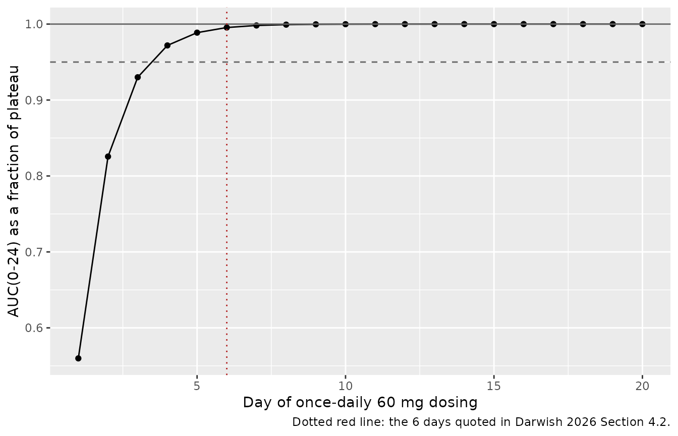
Dose proportionality (Figure 3)
Section 2.7 fits the power model
ln(Y) = intercept + beta * ln(dose) and declares
proportionality when the 90% CI of beta lies within
(1 + ln(0.8)/ln(r), 1 + ln(1.25)/ln(r)), with
r the ratio of the highest to the lowest dose. The packaged
model is structurally linear, so this reproduces the paper’s conclusion
by construction rather than as an independent test; it is included to
confirm that no dose-dependent term crept into the encoding.
doses_mg <- c(10, 20, 40, 60, 90, 120, 130, 180)

dp_events <- tidyr::expand_grid(dose_mg = doses_mg, time = seq(0, 25, by = 0.005)) |>
  dplyr::mutate(id = as.integer(factor(dose_mg)), evid = 0L,
                amt = NA_real_, cmt = "central") |>
  dplyr::bind_rows(
    tibble::tibble(dose_mg = doses_mg) |>
      dplyr::mutate(id = as.integer(factor(dose_mg)), time = 0, evid = 1L,
                    amt = dose_mg * 1000, cmt = "depot")
  ) |>
  dplyr::mutate(SEXF = 0L, FED = 0L) |>
  dplyr::arrange(id, time, dplyr::desc(evid))

dp <- rxode2::rxSolve(mod_typical, events = dp_events, keep = "dose_mg",
                      returnType = "data.frame") |>
  dplyr::group_by(dose_mg) |>
  dplyr::filter(time <= 1) |>
  dplyr::summarise(
    cmax    = max(Cc),
    auc0_24 = sum(diff(time) * (head(Cc, -1) + tail(Cc, -1)) / 2),
    .groups = "drop"
  )
#> ℹ omega/sigma items treated as zero: 'etalcl', 'etalvc', 'etalka', 'etaltlag'
#> Warning: multi-subject simulation without without 'omega'

r_ratio <- max(doses_mg) / min(doses_mg)
lo <- 1 + log(0.8) / log(r_ratio)
hi <- 1 + log(1.25) / log(r_ratio)

beta <- vapply(c(cmax = "cmax", auc0_24 = "auc0_24"), function(y) {
  unname(coef(lm(log(dp[[y]]) ~ log(dp$dose_mg)))[2])
}, numeric(1))

data.frame(
  parameter = c("Cmax", "AUC0-24"),
  beta = beta,
  criterion_low = lo,
  criterion_high = hi,
  within = beta > lo & beta < hi
) |>
knitr::kable(digits = 4, caption = "Dose-proportionality exponents (Figure 3 criterion).")| parameter | beta | criterion_low | criterion_high | within | |
|---|---|---|---|---|---|
| cmax | Cmax | 1 | 0.9228 | 1.0772 | TRUE |
| auc0_24 | AUC0-24 | 1 | 0.9228 | 1.0772 | TRUE |
Virtual cohort
Original observed data are not publicly available. Two virtual cohorts are used, each of 200 participants per arm.
- Analysis-like cohort – 200 participants with the sex balance (30.6% female) and fed-record fraction (29%) of the pooled analysis dataset (Supplemental Tables 2 and 3). Used for the post hoc parameter comparison against Table 2 and for the NCA validation.
- Simulation cohort – the 2 x 2 factorial of sex and fed status at 200 per cell, mirroring the 1:1 random assignment Darwish 2026 Section 2.6 used for its virtual population of 1000 (500 per group for each categorical covariate). Used for the steady-state exposure comparison.
# set.seed() seeds R's RNG, not rxode2's simulation RNG, and rxode2's streams
# are partitioned per solver thread -- so this cohort is reproducible on this
# machine and different on a machine with a different thread count. Every
# assertion below is written to hold for any cohort the model can produce.
set.seed(20260913)
rxode2::rxSetSeed(20260913)

expand_events <- function(subjects, dose_ug, dose_times, obs_times) {
  dosing <- tidyr::expand_grid(subjects, time = dose_times) |>
    dplyr::mutate(evid = 1L, amt = dose_ug, cmt = "depot")
  obs <- tidyr::expand_grid(subjects, time = obs_times) |>
    dplyr::mutate(evid = 0L, amt = NA_real_, cmt = "central")
  dplyr::bind_rows(dosing, obs) |>
    dplyr::arrange(id, time, dplyr::desc(evid))
}

n_arm <- 200L

# Analysis-like cohort: single 60 mg dose, followed to day 5.
subj_analysis <- tibble::tibble(
  id   = seq_len(n_arm),
  SEXF = as.integer(seq_len(n_arm) <= round(0.306 * n_arm)),
  FED  = as.integer(seq_len(n_arm) %% 100L < 29L),
  arm  = "Analysis-like"
)
ev_analysis <- expand_events(subj_analysis, 60000, 0, seq(0, 5, by = 0.02))

# Simulation cohort: 2 x 2 factorial, 60 mg once daily for 14 days.
subj_sim <- tidyr::expand_grid(SEXF = 0:1, FED = 0:1, k = seq_len(n_arm)) |>
  dplyr::mutate(
    id  = dplyr::row_number(),
    arm = paste0(ifelse(SEXF == 1, "Female", "Male"), ", ",
                 ifelse(FED == 1, "fed", "fasted"))
  ) |>
  dplyr::select(id, SEXF, FED, arm)

ev_sim <- expand_events(
  subj_sim, 60000,
  dose_times = 0:13,
  obs_times  = sort(unique(c(seq(0, 13, by = 0.25), seq(13, 14, by = 0.005))))
)

stopifnot(
  !anyDuplicated(unique(ev_analysis[, c("id", "time", "evid")])),
  !anyDuplicated(unique(ev_sim[, c("id", "time", "evid")])),
  nrow(dplyr::count(subj_sim, arm)) == 4L,
  all(dplyr::count(subj_sim, arm)$n == n_arm)
)
sim_analysis <- rxode2::rxSolve(mod, events = ev_analysis, keep = c("arm", "SEXF", "FED"),
                                returnType = "data.frame")
#> ℹ parameter labels from comments will be replaced by 'label()'
sim_ss <- rxode2::rxSolve(mod, events = ev_sim, keep = c("arm", "SEXF", "FED"),
                          returnType = "data.frame")
stopifnot(!anyNA(sim_analysis$Cc), !anyNA(sim_ss$Cc), all(sim_ss$Cc >= 0))
Replicate published figures
Figure 2 – concentration-time profiles stratified by food status and by sex
Figure 2 of Darwish 2026 is a prediction-corrected VPC of the pooled dataset stratified by fasted (A) versus fed (B) and by male (C) versus female (D). The panels below show the corresponding simulated median and 5th/95th percentiles over the first two days of once-daily 60 mg dosing.
sim_ss |>
  dplyr::filter(time <= 2) |>
  tidyr::pivot_longer(c(FED, SEXF), names_to = "stratum_var", values_to = "level") |>
  dplyr::mutate(
    stratum = dplyr::case_when(
      stratum_var == "FED"  & level == 0 ~ "A. Fasted",
      stratum_var == "FED"  & level == 1 ~ "B. Fed",
      stratum_var == "SEXF" & level == 0 ~ "C. Male",
      TRUE                               ~ "D. Female"
    )
  ) |>
  dplyr::group_by(stratum, time) |>
  dplyr::summarise(
    Q05 = quantile(Cc, 0.05), Q50 = median(Cc), Q95 = quantile(Cc, 0.95),
    .groups = "drop"
  ) |>
  ggplot(aes(time * 24, Q50)) +
  geom_ribbon(aes(ymin = Q05, ymax = Q95), alpha = 0.25, fill = "steelblue") +
  geom_line(colour = "steelblue4") +
  facet_wrap(~stratum) +
  scale_y_log10() +
  labs(x = "Time (h)", y = "Remlifanserin concentration (ng/mL)",
       caption = "Replicates the stratification of Figure 2 of Darwish 2026 (60 mg once daily).")
#> Warning in scale_y_log10(): log-10 transformation introduced infinite values.
#> log-10 transformation introduced infinite values.
#> log-10 transformation introduced infinite values.
#> log-10 transformation introduced infinite values.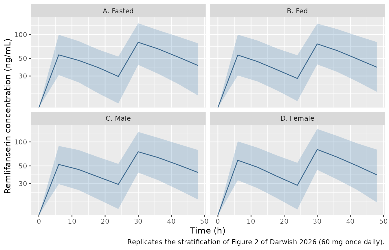
Table 2 – post hoc pharmacokinetic parameters
Table 2 summarises the post hoc PK parameters of the 209 analysed participants. Because the model’s random effects are log-normal, the expected values of these summaries are available in closed form, which makes this a deterministic comparison independent of any simulated draw. The analysis-like cohort’s empirical values are shown alongside for context but are not gated.
om <- c(cl = 0.1668, vc = 0.0981, ka = 0.3754, tlag = 0.01138)
cov_cl_vc <- 0.109
p_female  <- 0.306    # Supplemental Table 2
p_fed     <- 0.29     # Supplemental Table 3, record-weighted

e_vc_typ  <- 930 - 131 * p_female         # E[typical V/F] over the sex mixture
e_inv_vc  <- (1 - p_female) / 930 + p_female / 799
# etalcl and etalvc are correlated, so E[exp(etalcl - etalvc)] uses their
# combined variance: var(cl) + var(vc) - 2 * cov.
var_diff  <- om[["cl"]] + om[["vc"]] - 2 * cov_cl_vc

analytic <- c(
  `CL/F (L/day)` = 849 * exp(om[["cl"]] / 2),
  `V/F (L)`      = e_vc_typ * exp(om[["vc"]] / 2),
  `Kel (1/day)`  = 849 * e_inv_vc * exp(var_diff / 2),
  `T1/2 (h)`     = log(2) * 24 * (e_vc_typ / 849) * exp(var_diff / 2),
  `Ka (1/day)`   = 16.6 * exp(om[["ka"]] / 2),
  `ALAG1 (day)`  = 0.0300 * (1 + 0.290 * p_fed) * exp(om[["tlag"]] / 2)
)

published_mean <- c(`CL/F (L/day)` = 919.85, `V/F (L)` = 931.83,
                    `Kel (1/day)` = 0.98, `T1/2 (h)` = 17.75,
                    `Ka (1/day)` = 19.61, `ALAG1 (day)` = 0.0332)

per_subject <- sim_analysis |>
  dplyr::distinct(id, .keep_all = TRUE) |>
  dplyr::transmute(cl, vc, kel, t_half = log(2) / kel * 24, ka, tlag)

empirical_mean <- c(
  `CL/F (L/day)` = mean(per_subject$cl), `V/F (L)` = mean(per_subject$vc),
  `Kel (1/day)` = mean(per_subject$kel), `T1/2 (h)` = mean(per_subject$t_half),
  `Ka (1/day)` = mean(per_subject$ka),   `ALAG1 (day)` = mean(per_subject$tlag)
)

t2 <- data.frame(
  Parameter = names(published_mean),
  `Published mean (Table 2)` = unname(published_mean),
  `Model expected mean` = unname(analytic[names(published_mean)]),
  `Cohort mean (n = 200)` = unname(empirical_mean[names(published_mean)]),
  `% diff (analytic)` = unname(100 * (analytic[names(published_mean)] / published_mean - 1)),
  check.names = FALSE
)
knitr::kable(t2, digits = c(0, 4, 4, 4, 2),
caption = "Table 2 post hoc means vs. the model's closed-form expectations.")| Parameter | Published mean (Table 2) | Model expected mean | Cohort mean (n = 200) | % diff (analytic) |
|---|---|---|---|---|
| CL/F (L/day) | 919.8500 | 922.8431 | 899.3847 | 0.33 |
| V/F (L) | 931.8300 | 934.6525 | 903.8784 | 0.30 |
| Kel (1/day) | 0.9800 | 0.9815 | 0.9864 | 0.15 |
| T1/2 (h) | 17.7500 | 17.8509 | 17.6255 | 0.57 |
| Ka (1/day) | 19.6100 | 20.0274 | 19.9456 | 2.13 |
| ALAG1 (day) | 0.0332 | 0.0327 | 0.0329 | -1.48 |
# Structural gate: a mis-transcribed theta or a mis-scaled omega moves these by
# tens of percent. The closed-form column is deterministic, so a tight bound is
# appropriate here (it is not a random-cohort extreme).
stopifnot(max(abs(t2$`% diff (analytic)`)) < 5)
Every closed-form expectation lands within a few percent of the
published post hoc mean, which jointly confirms the thetas, the
covariate coefficients, the omega back-transform and the CL/V
covariance. Kel and T1/2 are the sharpest of
these: both depend on the CL/V covariance through
exp((var_cl + var_vc - 2 * cov) / 2), and would be visibly
wrong if the covariance had been dropped or its sign flipped.
Figure 4 – clinical relevance of the covariate effects
Figure 4 presents geometric mean ratios with 90% CIs for Cmax,ss and AUC0-24,ss against clinical-relevance bounds of 0.8 and 1.25. The paper’s conclusion is that “neither fed/fasted status nor sex exhibits a clinically relevant effect on steady-state remlifanserin exposures”.
tau_window <- function(d, lo = 13, hi = 14) dplyr::filter(d, time >= lo, time <= hi)

exposure <- sim_ss |>
  tau_window() |>
  dplyr::group_by(id, arm, SEXF, FED) |>
  dplyr::arrange(time, .by_group = TRUE) |>
  dplyr::summarise(
    cmax_ss = max(Cc),
    # ng/mL * day -> ng*h/mL
    auc_ss  = sum(diff(time) * (head(Cc, -1) + tail(Cc, -1)) / 2) * 24,
    .groups = "drop"
  )

gmr <- function(num, den) {
  lr <- log(num) - mean(log(den))
  n1 <- length(num); n2 <- length(den)
  s  <- sqrt(var(log(num)) / n1 + var(log(den)) / n2)
  m  <- mean(log(num)) - mean(log(den))
  c(gmr = exp(m), lower = exp(m - 1.645 * s), upper = exp(m + 1.645 * s))
}

contrasts <- dplyr::bind_rows(
  data.frame(metric = "Cmax,ss", contrast = "Fed / fasted",
             t(gmr(exposure$cmax_ss[exposure$FED == 1], exposure$cmax_ss[exposure$FED == 0]))),
  data.frame(metric = "AUC0-24,ss", contrast = "Fed / fasted",
             t(gmr(exposure$auc_ss[exposure$FED == 1], exposure$auc_ss[exposure$FED == 0]))),
  data.frame(metric = "Cmax,ss", contrast = "Female / male",
             t(gmr(exposure$cmax_ss[exposure$SEXF == 1], exposure$cmax_ss[exposure$SEXF == 0]))),
  data.frame(metric = "AUC0-24,ss", contrast = "Female / male",
             t(gmr(exposure$auc_ss[exposure$SEXF == 1], exposure$auc_ss[exposure$SEXF == 0])))
)

knitr::kable(contrasts, digits = 3,
caption = "Geometric mean ratios with 90% CIs (Figure 4 of Darwish 2026).")| metric | contrast | gmr | lower | upper |
|---|---|---|---|---|
| Cmax,ss | Fed / fasted | 1.003 | 0.960 | 1.047 |
| AUC0-24,ss | Fed / fasted | 1.007 | 0.961 | 1.056 |
| Cmax,ss | Female / male | 1.045 | 1.001 | 1.091 |
| AUC0-24,ss | Female / male | 0.997 | 0.951 | 1.046 |
ggplot(contrasts, aes(gmr, contrast)) +
  geom_vline(xintercept = 1, linetype = "solid", colour = "grey40") +
  geom_vline(xintercept = 0.8, linetype = "dashed", colour = "grey40") +
  geom_vline(xintercept = 1.25, linetype = "dashed", colour = "grey40") +
  geom_pointrange(aes(xmin = lower, xmax = upper)) +
  facet_wrap(~metric) +
  labs(x = "Geometric mean ratio (90% CI)", y = NULL,
       caption = "Replicates Figure 4 of Darwish 2026; dashed lines are the 0.8-1.25 bounds.")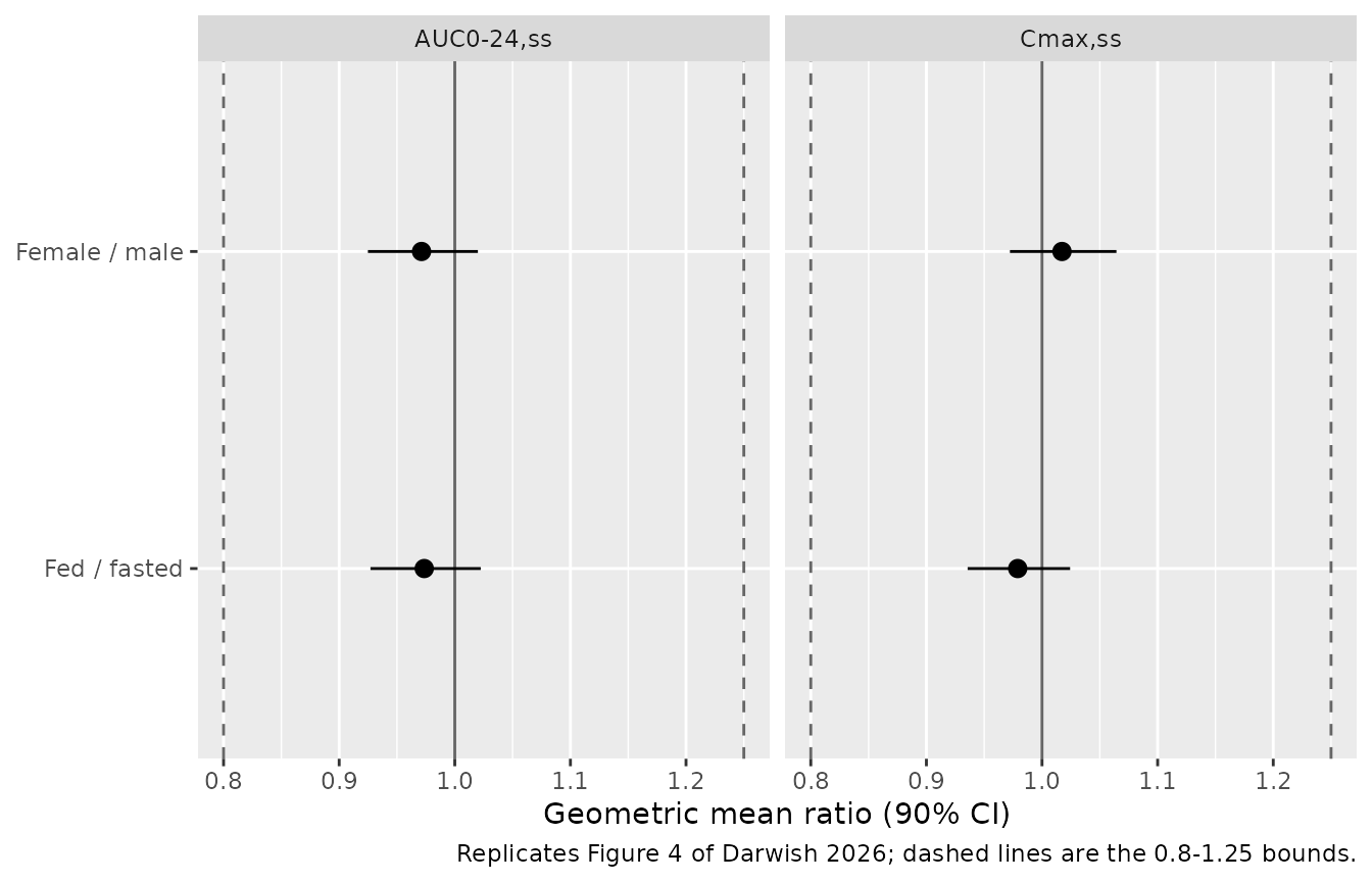
# The paper's own conclusion: every point estimate and 90% CI inside 0.8-1.25.
stopifnot(all(contrasts$lower > 0.8), all(contrasts$upper < 1.25))
The two mechanisms behind these ratios are worth stating explicitly,
because they are what makes the ratios insensitive to which cohort is
drawn. AUC0-24,ss is dose / (CL/F) for a linear
model at steady state, and neither covariate acts on CL/F, so both AUC
ratios are 1 up to sampling noise. Food acts only through the absorption
lag, which time-shifts a periodic steady state without changing its
peak, so the fed/fasted Cmax,ss ratio is also 1. The one
ratio that is genuinely non-unity is female/male Cmax,ss,
driven by the -131 L volume shift; it is the closest to a
bound and still comfortably inside it.
PKNCA validation
NCA is run on the analysis-like single-dose cohort using
Cc (the individual prediction, which carries no residual
error) so that the terminal slope is not corrupted by simulated assay
noise.
sim_nca <- sim_analysis |>
  dplyr::filter(!is.na(Cc)) |>
  # Per subject, keep Cc >= 1e-6 * Cmax after the peak: below that the ODE integrator has no relative accuracy left.
  dplyr::group_by(id) |>
  dplyr::filter(time <= time[which.max(Cc)] | Cc >= 1e-6 * max(Cc)) |>
  dplyr::ungroup() |>
  dplyr::select(id, time, Cc, arm)

# Guarantee a time = 0 row per subject; pre-dose Cc = 0 is correct for an
# extravascular dose.
sim_nca <- dplyr::bind_rows(
  sim_nca,
  sim_nca |> dplyr::distinct(id, arm) |> dplyr::mutate(time = 0, Cc = 0)
) |>
  dplyr::distinct(id, arm, time, .keep_all = TRUE) |>
  dplyr::arrange(id, time)

conc_obj <- PKNCA::PKNCAconc(sim_nca, Cc ~ time | arm + id)

dose_df <- ev_analysis |>
  dplyr::filter(evid == 1) |>
  dplyr::select(id, time, amt, arm)
dose_obj <- PKNCA::PKNCAdose(dose_df, amt ~ time | arm + id)

intervals <- data.frame(
  start = 0, end = Inf,
  cmax = TRUE, tmax = TRUE, auclast = TRUE, aucinf.obs = TRUE, half.life = TRUE
)

nca_res <- PKNCA::pk.nca(PKNCA::PKNCAdata(conc_obj, dose_obj, intervals = intervals))

nca_wide <- as.data.frame(nca_res) |>
  dplyr::filter(PPTESTCD %in% c("cmax", "tmax", "auclast", "aucinf.obs", "half.life")) |>
  dplyr::group_by(PPTESTCD) |>
  dplyr::summarise(
    median = median(PPORRES, na.rm = TRUE),
    p10 = quantile(PPORRES, 0.10, na.rm = TRUE),
    p90 = quantile(PPORRES, 0.90, na.rm = TRUE),
    .groups = "drop"
  )
knitr::kable(nca_wide, digits = 4,
caption = "PKNCA results, 60 mg single oral dose (time in days).")| PPTESTCD | median | p10 | p90 |
|---|---|---|---|
| aucinf.obs | 72.2487 | 44.5477 | 124.5597 |
| auclast | 71.3440 | 44.4515 | 121.8180 |
| cmax | 58.4373 | 37.5249 | 96.4429 |
| half.life | 0.7171 | 0.5436 | 0.9385 |
| tmax | 0.2200 | 0.1400 | 0.3400 |
# Internal consistency: NCA AUCinf must recover dose / (CL/F) subject by
# subject. This is the strongest available check on the whole solve-and-NCA
# pipeline and holds exactly, not statistically.
auc_by_id <- as.data.frame(nca_res) |>
  dplyr::filter(PPTESTCD == "aucinf.obs") |>
  dplyr::select(id, aucinf = PPORRES) |>
  dplyr::left_join(dplyr::distinct(sim_analysis, id, cl), by = "id") |>
  dplyr::mutate(ratio = cl * aucinf / 60000)
cat(sprintf("CL/F * AUCinf / dose: median %.4f, range %.4f-%.4f\n",
            median(auc_by_id$ratio), min(auc_by_id$ratio), max(auc_by_id$ratio)))
#> CL/F * AUCinf / dose: median 1.0002, range 0.9993-1.0008
stopifnot(abs(median(auc_by_id$ratio) - 1) < 0.01,
          quantile(abs(auc_by_id$ratio - 1), 0.95) < 0.02)
Comparison against published NCA
Darwish 2026 reports no NCA Cmax or AUC values for the pooled dataset – its Table 2 is a summary of post hoc model parameters. The one parameter with a direct NCA analogue is the terminal half-life, whose published post hoc median is 17.45 h.
published_nca <- data.frame(arm = "Analysis-like", half.life = 17.45)

nca_hours <- as.data.frame(nca_res) |>
  dplyr::filter(PPTESTCD == "half.life") |>
  dplyr::mutate(PPORRES = PPORRES * 24)   # days -> hours

cmp <- nlmixr2lib::ncaComparisonTable(
  simulated = nca_hours,
  reference = published_nca,
  by = "arm",
  units = c(half.life = "h"),
  tolerance_pct = 20
)
knitr::kable(cmp, caption = "Simulated vs. published half-life. * differs by >20%.")| NCA parameter | arm | Reference | Simulated | % diff |
|---|---|---|---|---|
| t½ (h) | Analysis-like | 17.4 | 17.2 | -1.4% |
sim_half_life <- median(nca_hours$PPORRES, na.rm = TRUE)
cat(sprintf("Simulated median t1/2 %.2f h vs. published post hoc median 17.45 h (%.1f%%)\n",
            sim_half_life, 100 * (sim_half_life / 17.45 - 1)))
#> Simulated median t1/2 17.21 h vs. published post hoc median 17.45 h (-1.4%)
stopifnot(abs(sim_half_life / 17.45 - 1) < 0.10)
Assumptions and deviations
-
Interindividual variances were back-transformed, not
transcribed. Darwish 2026 Table 1 prints IIV only as a percent
CV. Each
ini()variance islog(1 + CV^2). The choice of scale is not an assumption: the “Pinning the omega scale” section above shows it is the only one of the two candidates that reproduces the Table 1 footnote’s r = 0.852 / r2 = 0.726, and the Supplemental Methods$OMEGAinitial estimates corroborate it independently. -
Values come from Table 1, not from the supplement’s
$THETAblock. The Supplemental Methods control stream is the initial-estimate version (THETA 845, 965, 16.7, 0.03, 0.289, -222;$SIGMA0.0389). Every packaged value is the final estimate from Table 1. The control stream was used only for the model structure – the additive-inside-the-eta placement of the sex effect on V/F, the proportional food effect on ALAG1,S2 = V, and the purely proportional$ERRORblock. -
Dose amounts are in micrograms. This follows the
control stream’s
S2=V ;Dose amount = ug; Volume = L; Concentration = ng/mLcomment. A 60 mg dose is entered as60000. Entering60instead would under-predict concentrations 1000-fold. -
Covariates screened but not retained are recorded, not
encoded. Age, weight, BMI, BSA, race, eGFR, renal-function
category, hepatic-function category, ALT, AST and total bilirubin were
all screened by Darwish 2026 Section 2.4 and dropped. They appear in the
model file’s
covariatesDataExcludedlist so the provenance of the covariate search is preserved without declaring unused covariates. The supplement’s$PKblock still computesRACEB,GFRCKDEP2andRFCAT2as leftovers of the stepwise search; none enters a parameter equation, so none is encoded here. - Fed status is a per-record covariate. Table 2’s footnote states that ALAG1 is non-stationary per participant and that some participants in the food-effect study had more than one distinct ALAG1 value. The virtual cohorts here assign one fed status per subject, which is adequate for the covariate contrasts but does not reproduce the within-subject crossover of study 010. The record-weighted fed fraction of 29% (Supplemental Table 3) was used for the closed-form ALAG1 expectation; Table 2’s own ALAG1 mean implies a fed fraction nearer 35% across its 242 records, which is the main reason the ALAG1 row of the Table 2 comparison is the least tight of the six.
-
Below-quantitation handling is not replicated.
Darwish 2026 excluded the 1.3% of samples below the 0.10 ng/mL LLOQ as
missing. Simulated
Ccvalues carry no assay noise and are never censored here, so the NCA terminal slope is estimated from a noiseless profile. This makes the half-life comparison a check on the model’sCL/Vratio rather than on the paper’s BLQ policy. - Post hoc estimates shrink; simulated parameters do not. The Table 2 comparison is therefore made on means and medians, where shrinkage has little effect, and not on standard deviations or on the min/max columns, where it has a large one.
- The dose-proportionality check is structural. A one-compartment linear model cannot produce a non-unity power exponent, so reproducing Figure 3’s conclusion confirms only that no dose-dependent term was introduced during encoding. It is not independent evidence for the paper’s finding.
-
No parameter was tuned. Every value in
ini()is a verbatim Table 1 estimate or a documented back-transform of one.