Teduglutide (Marier 2021)
Source:vignettes/articles/Marier_2021_teduglutide.Rmd
Marier_2021_teduglutide.RmdModel and source
- Citation: Marier JF, Jomphe C, Peyret T, Wang Y. Population pharmacokinetics and exposure-response analyses of teduglutide in adult and pediatric patients with short bowel syndrome. Clin Transl Sci. 2021;14(6):2497-2509. doi:10.1111/cts.13117
- Article: https://doi.org/10.1111/cts.13117
- PK model: One-compartment population PK model with first-order subcutaneous absorption and an absorption lag time for the GLP-2 analog teduglutide in adult and pediatric patients with short bowel syndrome (SBS) and in non-SBS subjects (healthy volunteers and subjects with renal or hepatic impairment), pooled from 17 studies (Marier 2021). Power effects of body weight on Ka, CL/F and Vc/F; power effects of capped creatinine clearance on CL/F and of age on Vc/F; categorical effects of disease status (non-SBS) and sex on CL/F; injection site (non-abdomen) on Ka, lag time and relative bioavailability; formulation strength and supra-therapeutic dose on lag time.
- Exposure-response model: Time- and exposure-response model for the change from baseline in weekly prescribed parenteral support volume (PPSV) in adult and pediatric patients with short bowel syndrome treated with the GLP-2 analog teduglutide (Marier 2021). The change approaches a maximum reduction Emax with a hyperbolic time course (ET50 = 168 days, fixed); Emax scales as a power function of the individual steady-state teduglutide Cmax, with separate multipliers on Emax for the placebo arm and the 0.10 mg/kg dose level. Algebraic model with no dose events: the steady-state Cmax is supplied as a covariate, for example from Marier_2021_teduglutide.
Teduglutide is a recombinant analog of human glucagon-like peptide-2 approved for patients with short bowel syndrome (SBS) who depend on parenteral support (PS). Marier 2021 reports two sequential analyses, packaged here as two model files that share this vignette:
-
Marier_2021_teduglutide– a population PK model fitted in NONMEM 7.4.3 to 17 studies (219 SBS patients from 4 months to 79 years, 259 non-SBS subjects). It is a one-compartment model with first-order subcutaneous absorption and a lag time, with estimated body-weight exponents on Ka, CL/F and Vc/F, and covariate effects of capped creatinine clearance, age, sex, disease status, injection site, vial strength and a supra-therapeutic dose. -
Marier_2021_teduglutide_ppsv– a time- and exposure-response model fitted in Phoenix NLME 8.0 to 4918 weekly prescribed PS volumes from 249 SBS patients. The change from baseline approaches a maximum reduction with a hyperbolic time course (ET50 fixed at 168 days), and the maximum reduction scales with the individual steady-state teduglutideCmaxpredicted by the PK model.
The parameter tables are in the online supplement (Table S8 for PK,
Table S10 for exposure-response), which also prints the final NONMEM
control stream (run7a). The control stream settles the covariate coding
and the (1 + theta) form of every categorical effect.
Population
The PK analysis (Results, ‘Baseline characteristics’; Tables S4 and S5) pooled 478 subjects: 25 Japanese SBS patients (14 adults, 11 pediatric), 194 non-Japanese SBS patients (106 adults, 88 pediatric) and 259 non-SBS subjects (healthy volunteers and subjects with renal or moderate hepatic impairment). Of the SBS patients, 5 were under 1 year, 86 were 1-11 years, 8 were 12-17 years and 120 were adults. Overall, 63.2% were male and 81.6% White; the median age was 34.5 years (range 0.380-80.0) and the median weight 65.5 kg (range 5.15-127). Median creatinine clearance was 99.4 mL/min; 72.4% had normal renal function, 16.3% mild, 8.4% moderate and 1.5% severe impairment, and 1.3% had end-stage renal disease. SBS patients received 0.0125-0.15 mg/kg once daily; all Japanese patients received 0.05 mg/kg.
The exposure-response analysis used 249 SBS patients with a baseline PS volume from 10 studies, including the 2-year extension CL0600-021 that informed the time course.
Source trace
| Quantity | Value | Source |
|---|---|---|
| Structure: 1-compartment, first-order absorption, lag | – | Methods; supplement control stream $DES
|
| Ka | 0.330 1/h | Table S8 |
| CL/F | 16.0 L/h | Table S8 |
| Vc/F | 33.9 L | Table S8 |
| ALAG | 0.299 h | Table S8 |
| F1 | 1, fixed | Table S8; control stream 1 FIX ; TVF1
|
| WT on CL/F, Vc/F, Ka | 0.488, 1.35, -0.798 (reference 70 kg) | Table S8; control stream (WT/70)**THETA
|
| Capped CrCL on CL/F | 0.341 (reference 99.35 mL/min, cap 150) | Table S8 and footnote |
| Non-SBS on CL/F | x 0.668 | Table S8; control stream POP1
|
| Female on CL/F | x 0.932 | Table S8; control stream SEXN
|
| Age on Vc/F | -0.312 (reference 34 years) | Table S8; control stream VAGE
|
| Non-abdominal site on Ka, ALAG, F1 | x 0.766, x 1.458, x 0.936 | Table S8; control stream EXLOC1
|
| Vial strength >= 10 mg/vial on ALAG | x 0.476 | Table S8; control stream STRENGTH2
|
| Supra-therapeutic dose on ALAG | x 1.783 | Table S8; control stream SUPRA
|
| BSV CL/F, Vc/F, Ka | 22.1%, 30.5%, 22.9% CV | Table S8 |
| Residual error | 24.3% proportional + 6.51 ng/mL additive | Table S8; control stream $ERROR
|
E-R structure: Emax * t / (ET50 + t) * DrugEffect
|
– | Methods, ‘Exposure-response analysis’ |
| Emax | -5.76 L/week | Table S10 |
| ET50 | 168 days, fixed | Table S10 and note |
| Cmax exponent on Emax | 0.684 (reference 30 ng/mL, see below) | Table S10; Table S14 |
| Placebo effect on Emax | -0.276 | Table S10 |
| 0.10 mg/kg dose effect on Emax | -0.225 | Table S10 |
| E-R additive error | 1.11 L/week | Table S10 |
IIV round-trips to the published percentages
ini_pk <- rxode2::rxode(readModelDb("Marier_2021_teduglutide"))$iniDf
#> ℹ parameter labels from comments will be replaced by 'label()'
om <- ini_pk[!is.na(ini_pk$neta1) & ini_pk$neta1 == ini_pk$neta2, c("name", "est")]
om$cv_pct <- 100 * sqrt(exp(om$est) - 1)
om$published <- c(etalcl = 22.1, etalvc = 30.5, etalka = 22.9)[om$name]
knitr::kable(om, digits = 4, row.names = FALSE)| name | est | cv_pct | published |
|---|---|---|---|
| etalcl | 0.0477 | 22.1010 | 22.1 |
| etalvc | 0.0890 | 30.5002 | 30.5 |
| etalka | 0.0511 | 22.8995 | 22.9 |
Structural checks that need no cohort
The Results and Discussion print derived typical values that follow from the Table S8 parameters alone, so they check the transcription exactly.
th <- setNames(ini_pk$est, ini_pk$name)
t_half_typ <- log(2) * exp(th[["lvc"]]) / exp(th[["lcl"]])
# Discussion: 'typical subjects of 0.38 and 80 years of age ... are expected to
# have V/F values ... (137 L and 26.0 L, respectively) relative to a typical
# subject of 34 years of age (33.9 L)'.
v_age <- exp(th[["lvc"]]) * (c(0.38, 80, 34) / 34)^th[["e_age_vc"]]
checks <- data.frame(
  quantity = c("Typical t1/2 (h)", "Vc/F at 0.38 years (L)", "Vc/F at 80 years (L)", "Vc/F at 34 years (L)"),
  model = c(t_half_typ, v_age),
  published = c(1.47, 137, 26.0, 33.9)
)
checks$pct_diff <- 100 * (checks$model - checks$published) / checks$published
knitr::kable(checks, digits = 3)| quantity | model | published | pct_diff |
|---|---|---|---|
| Typical t1/2 (h) | 1.469 | 1.47 | -0.095 |
| Vc/F at 0.38 years (L) | 137.762 | 137.00 | 0.556 |
| Vc/F at 80 years (L) | 25.957 | 26.00 | -0.165 |
| Vc/F at 34 years (L) | 33.900 | 33.90 | 0.000 |
Virtual cohort
Table 1 of Marier 2021 summarises individual PK parameters and steady-state exposure for Japanese and non-Japanese adult and pediatric SBS patients on 0.05 mg/kg once daily. The paper does not publish the covariate distributions of those four subgroups, so the cohorts below are approximations built from the overall ranges of Table S5 (see “Assumptions and deviations”). Two non-Japanese cohorts are simulated, 200 adults and 200 children.
# rxSetSeed() fixes rxode2's draw on this machine only; its streams are
# partitioned per solver thread, so another machine draws a different cohort.
# Every assertion below is therefore on a cohort centre or a robust quantile.
set.seed(20260929)
rxode2::rxSetSeed(20260929)

n_per_arm <- 200L
tau <- 24
n_dose <- 3L
t_last <- (n_dose - 1L) * tau

make_cohort <- function(n, group, id_offset) {
  if (group == "Adult") {
    age <- stats::runif(n, 18, 79)
    wt <- pmin(pmax(stats::rlnorm(n, log(60), 0.22), 35), 110)
    crcl <- pmin(pmax(stats::rlnorm(n, log(85), 0.35), 26), 251)
  } else {
    # Age bands in the proportions of the 99 pediatric SBS patients of
    # Table S4: 5 under 1 year, 86 aged 1-11 years, 8 aged 12-17 years.
    band <- sample(1:3, n, replace = TRUE, prob = c(5, 86, 8))
    age <- stats::runif(n, c(0.38, 1, 12)[band], c(1, 12, 18)[band])
    # Children with SBS are frequently small for age. The weight-for-age line
    # is anchored to the median weight that Table 1 itself implies for the
    # non-Japanese pediatric group: AUCss = dose / (CL/F), so
    # 123 ng*h/mL x 7.08 L/h / (0.05 mg/kg x 1000) = 17.4 kg.
    wt <- pmin(pmax((6 + 1.8 * age) * stats::rlnorm(n, 0, 0.2), 5.15), 80)
    # Absolute (mL/min) clearance from a BSA-normalized eGFR of ~110
    # mL/min/1.73 m^2 scaled by a weight-based body-surface approximation.
    crcl <- 110 * (wt / 70)^0.7 * stats::rlnorm(n, 0, 0.25)
  }
  subj <- data.frame(
    id = id_offset + seq_len(n), group = group,
    AGE = age, WT = wt, CRCL = crcl,
    SEXF = stats::rbinom(n, 1, 0.44),
    DIS_SBS = 1L, INJSITE_ARM = 0L, INJSITE_THIGH = 0L,
    FORM_TEDUGLUTIDE_GE10MGVIAL = 0L, DOSE_HIGH = 0L
  )
  dose <- subj[rep(seq_len(n), each = n_dose), ]
  dose$time <- rep((seq_len(n_dose) - 1L) * tau, times = n)
  dose$amt <- 0.05 * dose$WT
  dose$evid <- 1L
  dose$cmt <- "depot"
  obs_grid <- t_last + c(0, seq(0.25, 12, by = 0.25), 14, 16, 18, 20, 22, 24)
  obs <- subj[rep(seq_len(n), each = length(obs_grid)), ]
  obs$time <- rep(obs_grid, times = n)
  obs$amt <- 0
  obs$evid <- 0L
  obs$cmt <- "central"
  dplyr::bind_rows(dose, obs) |> dplyr::arrange(id, time, dplyr::desc(evid))
}

events <- dplyr::bind_rows(
  make_cohort(n_per_arm, "Adult", 0L),
  make_cohort(n_per_arm, "Pediatric", n_per_arm)
)
stopifnot(!anyDuplicated(events[, c("id", "time", "evid")]))

events |>
  dplyr::distinct(id, group, AGE, WT, CRCL, SEXF) |>
  dplyr::group_by(group) |>
  dplyr::summarise(
    n = dplyr::n(), age_median = median(AGE), wt_median = median(WT),
    crcl_median = median(CRCL), female_pct = 100 * mean(SEXF)
  ) |>
knitr::kable(digits = 1)| group | n | age_median | wt_median | crcl_median | female_pct |
|---|---|---|---|---|---|
| Adult | 200 | 51.9 | 57.9 | 82.5 | 45 |
| Pediatric | 200 | 7.0 | 17.4 | 42.8 | 45 |
Simulation
mod_pk <- readModelDb("Marier_2021_teduglutide")
sim <- rxode2::rxSolve(mod_pk, events, keep = c("group"), returnType = "data.frame")
#> ℹ parameter labels from comments will be replaced by 'label()'
sim_ss <- sim |> dplyr::filter(time >= t_last)
Replicate published figures
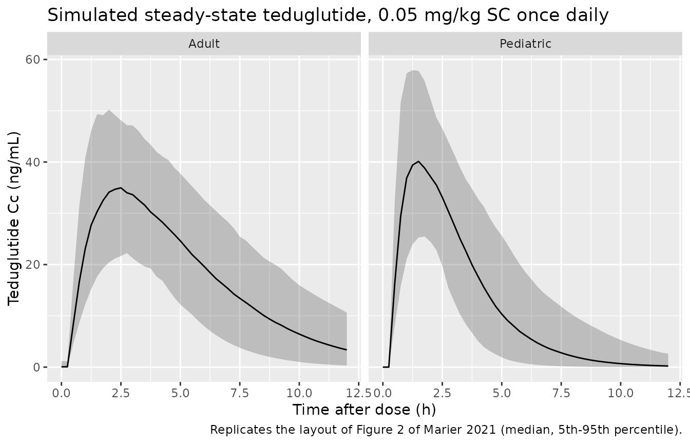
Figure 2 – steady-state profile over the first 12 hours after dosing
Figure 2 of Marier 2021 is a VPC of teduglutide concentrations up to 12 h post-dose in adult and pediatric SBS patients; peak concentrations sit at roughly 3-5 h post-dose and then decline rapidly (Results).
vpc <- sim_ss |>
  dplyr::mutate(tad = time - t_last) |>
  dplyr::filter(tad <= 12) |>
  dplyr::group_by(group, tad) |>
  dplyr::summarise(
    p05 = stats::quantile(Cc, 0.05), p50 = median(Cc), p95 = stats::quantile(Cc, 0.95),
    .groups = "drop"
  )
ggplot(vpc, aes(tad, p50)) +
  geom_ribbon(aes(ymin = p05, ymax = p95), alpha = 0.25) +
  geom_line() +
  facet_wrap(~group) +
  labs(
    x = "Time after dose (h)", y = "Teduglutide Cc (ng/mL)",
    title = "Simulated steady-state teduglutide, 0.05 mg/kg SC once daily",
    caption = "Replicates the layout of Figure 2 of Marier 2021 (median, 5th-95th percentile)."
  )
PKNCA validation
conc_df <- sim_ss |>
  dplyr::filter(!is.na(Cc)) |>
  dplyr::select(id, time, Cc, group) |>
  # The pre-dose trough of a fast-absorbing child can be ODE round-off of
  # order -1e-16 ng/mL, which PKNCA propagates to a NaN AUC; clamp it to 0.
  dplyr::mutate(Cc = pmax(Cc, 0))
# The interval starts at t_last, which is itself a simulated observation (the
# pre-dose trough), so every subject has an anchor row for AUC0-tau.
stopifnot(all(tapply(conc_df$time, conc_df$id, min) == t_last))

dose_df <- events |>
  dplyr::filter(evid == 1) |>
  dplyr::select(id, time, amt, group)

conc_obj <- PKNCA::PKNCAconc(conc_df, Cc ~ time | group + id, concu = "ng/mL", timeu = "h")
dose_obj <- PKNCA::PKNCAdose(dose_df, amt ~ time | group + id, doseu = "mg")
intervals <- data.frame(start = t_last, end = t_last + tau, cmax = TRUE, tmax = TRUE, auclast = TRUE)
nca_res <- PKNCA::pk.nca(PKNCA::PKNCAdata(conc_obj, dose_obj, intervals = intervals))
Comparison against Table 1 (non-Japanese SBS patients)
Table 1 reports medians of the model-predicted individual steady-state exposure. The comparison is on cohort medians; the simulated cohort approximates, rather than reproduces, the covariates of each subgroup, and the pediatric cohort is the less certain of the two: its simulated steady-state Cmax and AUC run about 20-30% above the Table 1 medians.
published <- data.frame(
  group = c("Adult", "Pediatric"),
  cmax = c(34.6, 32.5),
  auclast = c(203, 123)
)
cmp <- nlmixr2lib::ncaComparisonTable(
  simulated = nca_res,
  reference = published,
  by = "group",
  params = c("cmax", "auclast"),
  units = c(cmax = "ng/mL", auclast = "ng*h/mL"),
  tolerance_pct = 20
)
knitr::kable(cmp, caption = "Simulated steady-state NCA vs Marier 2021 Table 1 medians (non-Japanese). * flags a >20% difference.")| NCA parameter | group | Reference | Simulated | % diff |
|---|---|---|---|---|
| Cmax (ng/mL) | Adult | 34.6 | 36.3 | +5.0% |
| Cmax (ng/mL) | Pediatric | 32.5 | 41.3 | +27.0%* |
| AUClast (ng*h/mL) | Adult | 203 | 229 | +12.6% |
| AUClast (ng*h/mL) | Pediatric | 123 | 149 | +21.5%* |
The individual-parameter summaries of Table 1 are compared the same
way. The half-life in Table 1 is the model-derived
ln(2) * V/F / (CL/F); a PKNCA terminal half-life would
instead estimate the slower absorption phase, because Ka (about 0.4 1/h
in adults) is smaller than the elimination rate constant (about 0.6
1/h), so the model-derived quantity is compared.
indiv <- sim_ss |>
  dplyr::distinct(id, group, ka, cl, vc) |>
  dplyr::mutate(thalf = log(2) * vc / cl)
param_cmp <- indiv |>
  dplyr::group_by(group) |>
  dplyr::summarise(ka = median(ka), cl = median(cl), vc = median(vc), thalf = median(thalf)) |>
  tidyr::pivot_longer(-group, names_to = "parameter", values_to = "simulated") |>
  dplyr::left_join(
    data.frame(
      group = rep(c("Adult", "Pediatric"), each = 4),
      parameter = rep(c("ka", "cl", "vc", "thalf"), 2),
      published = c(0.380, 14.3, 25.0, 1.28, 0.839, 7.08, 10.0, 1.02)
    ),
    by = c("group", "parameter")
  ) |>
  dplyr::mutate(pct_diff = 100 * (simulated - published) / published)
param_cmp |>
  dplyr::rename(
    Group = group, Parameter = parameter, `Simulated median` = simulated,
    `Table 1 median` = published, `% difference` = pct_diff
  ) |>
knitr::kable(digits = 3)| Group | Parameter | Simulated median | Table 1 median | % difference |
|---|---|---|---|---|
| Adult | ka | 0.376 | 0.380 | -1.107 |
| Adult | cl | 13.010 | 14.300 | -9.018 |
| Adult | vc | 25.507 | 25.000 | 2.027 |
| Adult | thalf | 1.335 | 1.280 | 4.318 |
| Pediatric | ka | 0.952 | 0.839 | 13.486 |
| Pediatric | cl | 5.844 | 7.080 | -17.464 |
| Pediatric | vc | 8.927 | 10.000 | -10.727 |
| Pediatric | thalf | 1.086 | 1.020 | 6.442 |
sim_wide <- as.data.frame(nca_res) |>
  dplyr::filter(PPTESTCD %in% c("cmax", "auclast")) |>
  dplyr::group_by(group, PPTESTCD) |>
  dplyr::summarise(median = median(PPORRES), .groups = "drop") |>
  tidyr::pivot_wider(names_from = PPTESTCD, values_from = median)
gate <- published |>
  dplyr::rename(cmax_pub = cmax, auclast_pub = auclast) |>
  dplyr::inner_join(sim_wide, by = "group") |>
  dplyr::mutate(
    cmax_pct = 100 * (cmax - cmax_pub) / cmax_pub,
    auc_pct = 100 * (auclast - auclast_pub) / auclast_pub
  )
stopifnot(
  nrow(gate) == 2L, !anyNA(gate$cmax_pct), !anyNA(gate$auc_pct),
  nrow(param_cmp) == 8L, !anyNA(param_cmp$pct_diff)
)
# Cohort centres against approximate covariate distributions. The adult
# covariates are well constrained by Table S5, so the adult bound is 20%. The
# pediatric weight, age and creatinine-clearance distributions are not
# published (see "Assumptions and deviations"), so the pediatric bound is 40%.
# A mis-transcribed weight exponent or clearance moves the pediatric centre by
# far more than that: a sign error on the Ka weight exponent alone moves
# pediatric Ka about 4-fold.
tol <- c(Adult = 20, Pediatric = 40)
stopifnot(
  all(abs(gate$cmax_pct) < tol[gate$group]),
  all(abs(gate$auc_pct) < tol[gate$group]),
  all(abs(param_cmp$pct_diff) < tol[param_cmp$group])
)
The steady-state AUC over the dosing interval is also a mass-balance
check: for linear PK, AUC0-tau equals
F * Dose / (CL/F) for every subject.
mb <- as.data.frame(nca_res) |>
  dplyr::filter(PPTESTCD == "auclast") |>
  dplyr::select(id, auclast = PPORRES) |>
  dplyr::inner_join(sim_ss |> dplyr::distinct(id, cl, fdepot), by = "id") |>
  dplyr::inner_join(dose_df |> dplyr::distinct(id, amt), by = "id") |>
  dplyr::mutate(pct = 100 * (auclast - 1000 * fdepot * amt / cl) / (1000 * fdepot * amt / cl))
stopifnot(nrow(mb) == 2L * n_per_arm)
# Same drawn parameters on both sides; the residual is trapezoidal error on the
# 15-minute grid plus the small carry-over from the previous dose.
stopifnot(abs(median(mb$pct)) < 3, stats::quantile(abs(mb$pct), 0.9) < 5)
Exposure-response: change from baseline in prescribed PS volume
The exposure-response model is algebraic in time. Its drug-effect
multiplier depends on the arm: placebo subjects take
1 + (-0.276), subjects on 0.10 mg/kg take
1 + (-0.225), and every other actively treated subject
takes (Cmax / 30)^0.684.
mod_er <- readModelDb("Marier_2021_teduglutide_ppsv")
# The published exposure-response model has no between-subject variability, so
# rxode2 notes that a multi-subject solve has no omega. That is expected here;
# muffle exactly that message and let any other warning through.
muffle_no_omega <- function(w) {
  if (grepl("without 'omega'", conditionMessage(w), fixed = TRUE)) invokeRestart("muffleWarning")
}
solve_er <- function(...) {
  withCallingHandlers(rxode2::rxSolve(...), warning = muffle_no_omega)
}
er_ev <- data.frame(
  id = 1:4, arm = c("Cmax 30 ng/mL", "Cmax 60 ng/mL", "Placebo", "0.10 mg/kg"),
  CMAX = c(30, 60, 0, 0), PLACEBO = c(0L, 0L, 1L, 0L), DOSE_HIGH = c(0L, 0L, 0L, 1L)
)
er_ev <- er_ev[rep(1:4, each = 3), ]
er_ev$time <- rep(c(168, 730, 1e6), times = 4)
er_ev$evid <- 0L
er_typ <- solve_er(mod_er, er_ev, keep = "arm", returnType = "data.frame")
er_tab <- er_typ |>
  dplyr::select(arm, time, ppsvcfb) |>
  tidyr::pivot_wider(names_from = time, values_from = ppsvcfb, names_prefix = "day_")
knitr::kable(er_tab, digits = 3, caption = "Typical change from baseline in PPSV (L/week).")| arm | day_168 | day_730 | day_1e+06 |
|---|---|---|---|
| Cmax 30 ng/mL | -2.880 | -4.682 | -5.759 |
| Cmax 60 ng/mL | -4.627 | -7.523 | -9.252 |
| Placebo | -2.085 | -3.390 | -4.170 |
| 0.10 mg/kg | -2.232 | -3.629 | -4.463 |
# Abstract: 'Daily dosing of 0.05 mg/kg teduglutide resulted in a maximum
# reduction in PS of 5.76 L/week' -- the plateau at the 30 ng/mL reference.
plateau_30 <- er_typ$ppsvcfb[er_typ$arm == "Cmax 30 ng/mL" & er_typ$time == 1e6]
day168_30 <- er_typ$ppsvcfb[er_typ$arm == "Cmax 30 ng/mL" & er_typ$time == 168]
plateau_pl <- er_typ$ppsvcfb[er_typ$arm == "Placebo" & er_typ$time == 1e6]
plateau_hi <- er_typ$ppsvcfb[er_typ$arm == "0.10 mg/kg" & er_typ$time == 1e6]
stopifnot(
  abs(plateau_30 - (-5.76)) < 0.01,
  # t = ET50 gives exactly half the plateau; Table 2 shows the same 1:2 ratio
  # between its week-24 and steady-state rows in every column.
  abs(day168_30 / plateau_30 - 0.5) < 1e-3,
  abs(plateau_pl - (-5.76 * (1 - 0.276))) < 0.01,
  abs(plateau_hi - (-5.76 * (1 - 0.225))) < 0.01
)
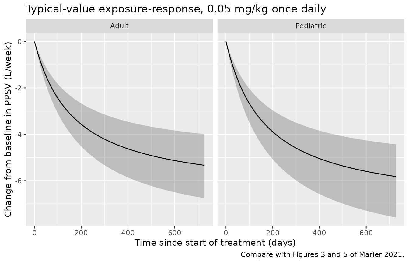
Feeding the individual steady-state Cmax of the
simulated PK cohorts into the exposure-response model gives a time
course for each subject. The published model reports no between-subject
variability, so the spread below comes from exposure alone.
cmax_i <- as.data.frame(nca_res) |>
  dplyr::filter(PPTESTCD == "cmax") |>
  dplyr::select(id, group, CMAX = PPORRES)
er_times <- c(0, seq(14, 728, by = 14))
er_cohort <- cmax_i[rep(seq_len(nrow(cmax_i)), each = length(er_times)), ]
er_cohort$time <- rep(er_times, times = nrow(cmax_i))
er_cohort$PLACEBO <- 0L
er_cohort$DOSE_HIGH <- 0L
er_cohort$evid <- 0L
er_sim <- solve_er(mod_er, er_cohort, keep = "group", returnType = "data.frame")

er_sim |>
  dplyr::group_by(group, time) |>
  dplyr::summarise(
    p05 = stats::quantile(ppsvcfb, 0.05), p50 = median(ppsvcfb), p95 = stats::quantile(ppsvcfb, 0.95),
    .groups = "drop"
  ) |>
  ggplot(aes(time, p50)) +
  geom_ribbon(aes(ymin = p05, ymax = p95), alpha = 0.25) +
  geom_line() +
  facet_wrap(~group) +
  labs(
    x = "Time since start of treatment (days)", y = "Change from baseline in PPSV (L/week)",
    title = "Typical-value exposure-response, 0.05 mg/kg once daily",
    caption = "Compare with Figures 3 and 5 of Marier 2021."
  )
er_ss <- er_sim |>
  dplyr::filter(time %in% c(168, 728)) |>
  dplyr::group_by(group, time) |>
  dplyr::summarise(median = median(ppsvcfb), .groups = "drop")
knitr::kable(er_ss, digits = 2, caption = "Median simulated change from baseline in PPSV (L/week).")| group | time | median |
|---|---|---|
| Adult | 168 | -3.28 |
| Adult | 728 | -5.34 |
| Pediatric | 168 | -3.58 |
| Pediatric | 728 | -5.82 |
Table 2 of Marier 2021 prints subgroup means and medians of the
individual predicted change from baseline (for example, non-Japanese
pediatric patients: median -2.12 L/week at week 24 and -4.25 L/week at
steady state). Those values come from individual fits whose random
effects are not reported, and their CVs of 78-148% cannot arise from
Cmax variation alone, so they are shown for orientation
only and are not used as a gate.
Assumptions and deviations
-
OMEGA covariances not reported. The final control
stream estimates a full 3 x 3 OMEGA block on CL/F, Vc/F and Ka, but
Table S8 reports only the variances (as %CV). The packaged model has a
diagonal OMEGA. The %CV values are converted with
omega^2 = log(CV^2 + 1), the lognormal relationship for the exponential random effects the Methods describe. -
Control-stream
$THETAvalues are initial estimates. The supplement’s control stream carries initial values (for exampleWTCL 0.510326,WTKA -0.561455); every packaged value comes from Table S8. -
Creatinine clearance cap. The source column CRCLT
is ‘estimated creatinine clearance rate capped at 150 mL/min’. The
packaged model applies the cap itself (
min(CRCL, 150)), so supply the uncapped value in mL/min (Cockcroft-Gault above 12 years; the modified Schwartz estimate converted to mL/min below 12 years). - Missing injection site. 24 SBS patients had no recorded injection site (Table S4); the paper does not say how they were coded. Supply the actual site.
-
Supra-therapeutic dose.
DOSE_HIGH = 1in the PK model stands for the 20 mg supra-therapeutic dose named in the Methods (‘therapeutic vs. supra-therapeutic [20 mg]’); whether other >= 20 mg phase 1 doses were flagged is not stated. -
Reference Cmax of the exposure-response model.
Table S10 gives the exponent of the Cmax effect (0.684) without the
normalizing concentration. The packaged model uses 30 ng/mL, the value
printed in the authors’ raw-PPSV sensitivity model of the same analysis
(Table S14,
(Cmax/30)^0.507). It is consistent with the Abstract’s statement that 0.05 mg/kg gives a maximum reduction of 5.76 L/week, since the median steady-stateCmaxat that dose is about 27-47 ng/mL across subgroups (Table 1). -
Stratified drug effect. The placebo and 0.10 mg/kg
multipliers replace, rather than multiply, the Cmax term, following
Table S14’s statement that the Cmax term applies ‘if dose < 0.1 mg/kg
and not placebo’. The multipliers are read as
1 + theta, the form the analysis uses for every categorical effect. - No exposure-response IIV. Table S10 reports no between-subject variability, so none is packaged. Table 2’s wide individual spread shows the fitted model carried random effects that were not published.
- Sensitivity models not packaged. Tables S11-S13 (fixed allometric exponents, renal maturation function) and Table S14 (raw PPSV with a baseline) are sensitivity analyses; only the final models are packaged.
- Virtual cohort. The subgroup covariate distributions behind Table 1 are not published. The adult and pediatric cohorts here approximate them from the overall ranges of Table S5, with an assumed pediatric weight-for-age and creatinine-clearance relationship, abdominal injection and vial strength below 10 mg/vial. The pediatric weight-for-age line is anchored to the 17.4 kg median weight implied by Table 1 (median AUCss x median CL/F / dose per kg). The Table 1 comparison is therefore a check of the cohort centre (20% tolerance for adults, 40% for children), not an exact reproduction.
- Inconsistent Table 2. The Results text and Table 2 disagree on which column holds which subgroup (for example, the text gives baseline PS volumes of 15.6 and 10.1 L/week for Japanese and non-Japanese adults, whereas the table places 10.1 L/week under non-Japanese pediatrics). Table 2 is not used for validation.
- No erratum. No correction to Marier 2021 was found in Europe PMC (checked 2026-09-29).