Model and source
- Citation: Zhu L, Li H, Chan P, Eley T, Gandhi Y, Bifano M, Osawa M, Ueno T, Hughes E, AbuTarif M, Bertz R, Garimella T. (2018). Population Pharmacokinetic Analysis of Asunaprevir in Subjects with Hepatitis C Virus Infection. Infectious Diseases and Therapy 7(2):261-275. doi:10.1007/s40121-018-0197-y.
- Article: https://doi.org/10.1007/s40121-018-0197-y
Asunaprevir (ASV, BMS-650032) is a twice-daily pangenotypic hepatitis C virus NS3 protease inhibitor. Zhu et al. pooled 9496 concentration records from 1236 subjects across three Phase II and two Phase III studies in which ASV was given with daclatasvir (the DUAL regimen) or with daclatasvir plus peginterferon/ribavirin (the QUAD regimen), and fitted a two-compartment model with sequential zero-order-then-first-order absorption and first-order elimination.
Three features of the fit drive everything this vignette checks:
-
Auto-induction of apparent clearance. CL/F is
multiplied by
exp(0.355) = 1.43from 48 h after the first dose onward, taking it from 50.8 to 72.5 L/h. The authors modelled this as a step rather than a continuous onset because the pooled dataset held almost no samples in the first week of dosing, so the induction dynamics were not estimable. A 6-day change point was also tried and gave a worse objective function. - Hepatic function as the dominant covariate axis. CL/F carries both a time-fixed baseline-AST term and a time-varying on-treatment AST/baseline ratio, plus a cirrhosis indicator. As antiviral treatment clears the virus, transaminases normalise and modelled clearance rises.
-
Formulation and dose level acting on absorption.
The Phase II tablet is absorbed more slowly
(
ka * exp(-0.503)), over a longer zero-order release (D1 * exp(0.864)), and less completely (F * exp(-0.215)) than the Phase III / commercial soft-gel capsule, and the 600 mg level carries a further bioavailability increment capturing the observed more-than-dose-proportional exposure.
cat(strwrap(mod_meta$description, width = 78), sep = "\n")
#> Two-compartment population PK model for asunaprevir (ASV, BMS-650032; a
#> pangenotypic hepatitis C virus NS3 protease inhibitor) in 1239 adults with
#> chronic HCV genotype 1 or 4 infection, pooled from 3 Phase II and 2 Phase III
#> studies in which ASV was given with daclatasvir (DUAL) or with daclatasvir
#> plus peginterferon/ribavirin (QUAD). Absorption is sequential: a zero-order
#> release from the formulation over a duration D1 into the depot, followed by
#> first-order absorption (ka) into the central compartment; elimination is
#> first order from central. Apparent clearance (CL/F) carries a step-function
#> auto-induction effect that raises CL/F by 43% (50.8 to 72.5 L/h) from 48 h
#> after the first dose onward, attributed to CYP3A4 auto-induction; the
#> induction dynamics themselves were not estimable because the pooled dataset
#> held few samples in the first 7 days. CL/F additionally depends on age, sex,
#> race (Black, Asian and Other relative to a White reference), baseline AST,
#> the on-treatment AST/baseline-AST ratio (a time-varying hepatic-recovery
#> term) and cirrhosis; Vc/F on sex and cirrhosis; Vp/F on body weight; and ka,
#> the zero-order duration D1 and relative bioavailability on the formulation
#> (Phase II tablet versus the Phase III / commercial soft-gel capsule
#> reference), with an additional bioavailability increment at the 600 mg dose
#> level that captures the observed more-than-dose-proportional exposure.
#> Inter-individual variability is diagonal on CL/F, Vc/F, Vp/F and ka, and
#> residual variability is additive on log-transformed concentrations (i.e.
#> log-normal).
Population
pop <- mod_ui$population
tibble::tibble(
  Field = names(pop),
  Value = vapply(pop, function(x) paste(
    if (is.null(names(x))) x else paste0(names(x), " ", x, "%"),
    collapse = "; "
  ), character(1))
) |>
knitr::kable()| Field | Value |
|---|---|
| species | human |
| n_subjects | 1239 |
| n_studies | 5 |
| age_range | 18-79 years |
| age_median | 57 years |
| weight_range | 36-124 kg |
| weight_median | 70 kg |
| sex_female_pct | 50.8 |
| race_ethnicity | White 58.3%; Black 6%; Asian 34.2%; Other 1.6% |
| disease_state | Chronic hepatitis C virus genotype 1 (98.5%) or genotype 4 (1.5%) infection; 19.5% with compensated cirrhosis; mild hepatic impairment (Child-Pugh A) permitted; treatment-naive (33.5%), non-responder or null/partial responder (35.1%), or peginterferon/ribavirin ineligible/intolerant (31.4%) |
| dose_range | 100, 200 or 600 mg once daily (4.3% of subjects) or twice daily (95.7%), as the Phase II tablet (30.3%) or the Phase III / commercial soft-gel capsule (69.7%); 69.7% received 100 mg BID soft-gel |
| regions | Global, including a Japanese Phase II and a Japanese Phase III study |
| hepatic_function | Baseline AST median 51 U/L (range 13-595); baseline ALT median 60 U/L (range 7-475); both roughly twice the upper limit of normal on average and falling by about 50% over the first 6 weeks of treatment |
| renal_function | Creatinine clearance median 101 mL/min (range 40-286) |
| co_medication | Daclatasvir in all subjects; peginterferon alfa and/or ribavirin in the QUAD and triple regimens |
| n_observations | 9496 |
| notes | Demographics from Zhu 2018 Table 1 (n = 1239). The final PK analysis dataset held 9496 concentration records from 1236 subjects (Results); most subjects contributed 4-9 samples. The five contributing studies are listed in Supplemental Table 1 of the Electronic Supplementary Material. |
The reference subject used throughout Zhu 2018 Table 2 and Figure 3, and used as the anchor for every deterministic check below, is a non-cirrhotic, male, 70 kg, 55-year-old White subject with baseline AST 60 IU/L receiving the soft-gel capsule, prior to induction.
Source trace
Every ini() value and every model()
equation, with its location in the source.
tibble::tribble(
  ~Quantity,                          ~Value,            ~`Source location`,
  "CL/F (pre-induction)",             "50.8 L/h",        "Table 2, 'CL/F (L/h)'",
  "Vc/F",                             "47.6 L",          "Table 2, 'Vc/F (L)'",
  "Q/F",                              "21.6 L/h",        "Table 2, 'Q/F (L/h)'",
  "Vp/F",                             "561 L",           "Table 2, 'Vp/F (L)'",
  "ka",                               "0.484 /h",        "Table 2, 'Ka (1/h)'",
  "D1 (zero-order release)",          "1.12 h",          "Table 2, 'D1 (h)'",
  "F (soft-gel, <600 mg)",            "1 (anchor)",      "Eq. for F; reference level of both indicators",
  "Auto-induction on CL/F",           "+0.355 (log)",    "Table 2, 'CL/F * induction'; Eq. for CL/F, I(Time > 48)",
  "Age on CL/F",                      "-0.341 (power)",  "Table 2, 'CL * age'; Eq. for CL/F, (Age/55)",
  "Female on CL/F",                   "-0.117 (log)",    "Table 2, 'CL * female'",
  "Black race on CL/F",               "+0.0386 (log)",   "Table 2, 'CL * Black Race'",
  "Asian race on CL/F",               "-0.255 (log)",    "Table 2, 'CL * Asian Race'",
  "Other race on CL/F",               "-0.0678 (log)",   "Table 2, 'CL * Other Race'",
  "Baseline AST on CL/F",             "-0.458 (power)",  "Eq. for CL/F, (Baseline AST/60)^-0.458; Table 2 prints the rounded -0.46",
  "AST/baseline AST on CL/F",         "-0.291 (power)",  "Eq. for CL/F, (AST/Baseline AST)^-0.291; Table 2 prints the rounded -0.29",
  "Cirrhosis on CL/F",                "-0.378 (log)",    "Table 2, 'CL * cirrhosis'",
  "Female on Vc/F",                   "-0.608 (log)",    "Table 2, 'Vc * female'; Eq. for Vc/F",
  "Cirrhosis on Vc/F",                "-0.835 (log)",    "Table 2, 'Vc * cirrhosis'; Eq. for Vc/F",
  "Weight on Vp/F",                   "+1.42 (power)",   "Table 2, 'Vp * weight'; Eq. for Vp/F, (Weight/70)",
  "Tablet on ka",                     "-0.503 (log)",    "Table 2, 'Ka * tablet'; Eq. for Ka",
  "Tablet on D1",                     "+0.864 (log)",    "Table 2, 'D1 * tablet'; Eq. for D",
  "Tablet on F",                      "-0.215 (log)",    "Table 2, 'Relative F * tablet'; Eq. for F",
  "600 mg level on F",                "+0.65 (log)",     "Table 2, 'Relative F1 * 600 mg'; Eq. for F",
  "IIV CL/F",                         "var 0.168",       "Table 2, random effect 'CL/F' (SD 0.41)",
  "IIV Vc/F",                         "var 2.19",        "Table 2, random effect 'Vc/F' (SD 1.48)",
  "IIV Vp/F",                         "var 0.777",       "Table 2, random effect 'Vp/F' (SD 0.881)",
  "IIV ka",                           "var 0.300",       "Table 2, random effect 'Ka' (SD 0.548)",
  "Residual (log-additive) SD",       "0.621",           "Table 2, residual error 'e' (variance 0.386)"
) |>
knitr::kable()| Quantity | Value | Source location |
|---|---|---|
| CL/F (pre-induction) | 50.8 L/h | Table 2, ‘CL/F (L/h)’ |
| Vc/F | 47.6 L | Table 2, ‘Vc/F (L)’ |
| Q/F | 21.6 L/h | Table 2, ‘Q/F (L/h)’ |
| Vp/F | 561 L | Table 2, ‘Vp/F (L)’ |
| ka | 0.484 /h | Table 2, ‘Ka (1/h)’ |
| D1 (zero-order release) | 1.12 h | Table 2, ‘D1 (h)’ |
| F (soft-gel, <600 mg) | 1 (anchor) | Eq. for F; reference level of both indicators |
| Auto-induction on CL/F | +0.355 (log) | Table 2, ‘CL/F * induction’; Eq. for CL/F, I(Time > 48) |
| Age on CL/F | -0.341 (power) | Table 2, ‘CL * age’; Eq. for CL/F, (Age/55) |
| Female on CL/F | -0.117 (log) | Table 2, ‘CL * female’ |
| Black race on CL/F | +0.0386 (log) | Table 2, ‘CL * Black Race’ |
| Asian race on CL/F | -0.255 (log) | Table 2, ‘CL * Asian Race’ |
| Other race on CL/F | -0.0678 (log) | Table 2, ‘CL * Other Race’ |
| Baseline AST on CL/F | -0.458 (power) | Eq. for CL/F, (Baseline AST/60)^-0.458; Table 2 prints the rounded -0.46 |
| AST/baseline AST on CL/F | -0.291 (power) | Eq. for CL/F, (AST/Baseline AST)^-0.291; Table 2 prints the rounded -0.29 |
| Cirrhosis on CL/F | -0.378 (log) | Table 2, ‘CL * cirrhosis’ |
| Female on Vc/F | -0.608 (log) | Table 2, ‘Vc * female’; Eq. for Vc/F |
| Cirrhosis on Vc/F | -0.835 (log) | Table 2, ‘Vc * cirrhosis’; Eq. for Vc/F |
| Weight on Vp/F | +1.42 (power) | Table 2, ‘Vp * weight’; Eq. for Vp/F, (Weight/70) |
| Tablet on ka | -0.503 (log) | Table 2, ‘Ka * tablet’; Eq. for Ka |
| Tablet on D1 | +0.864 (log) | Table 2, ‘D1 * tablet’; Eq. for D |
| Tablet on F | -0.215 (log) | Table 2, ‘Relative F * tablet’; Eq. for F |
| 600 mg level on F | +0.65 (log) | Table 2, ‘Relative F1 * 600 mg’; Eq. for F |
| IIV CL/F | var 0.168 | Table 2, random effect ‘CL/F’ (SD 0.41) |
| IIV Vc/F | var 2.19 | Table 2, random effect ‘Vc/F’ (SD 1.48) |
| IIV Vp/F | var 0.777 | Table 2, random effect ‘Vp/F’ (SD 0.881) |
| IIV ka | var 0.300 | Table 2, random effect ‘Ka’ (SD 0.548) |
| Residual (log-additive) SD | 0.621 | Table 2, residual error ‘e’ (variance 0.386) |
The two covariate equations are printed in the body of the paper
between Table 2 and the Model Evaluations heading (pp. 266-267). Three
of the covariate columns are new canonical entries registered with this
model: AST_BL (the time-fixed baseline AST anchor paired
with the time-varying AST), DIS_CIRRHOSIS, and
DOSE_600MG.
Event-table helper
Doses enter the depot compartment as a
zero-order release over D1 hours. rxode2
only honours dur(depot) when the dose record carries
rate = -2; without it the dose is delivered as a bolus and
D1 is silently ignored. A check below proves the duration
is actually engaged.
# Zhu 2018 Table 2 footnote a reference subject.
ref_cov <- list(
  AGE = 55, WT = 70, SEXF = 0,
  RACE_BLACK = 0, RACE_ASIAN = 0, RACE_OTHER = 0,
  AST_BL = 60, AST = 60, DIS_CIRRHOSIS = 0,
  FORM_TABLET = 0, DOSE_600MG = 0
)

make_events <- function(cov, dose = 100, ii = 12, n_dose = 30,
                        t_max = 15 * 24, by = 0.05, id = 1L) {
  dosing <- data.frame(
    id = id, time = seq(0, by = ii, length.out = n_dose),
    amt = dose, evid = 1L,
    # The ODE state, never the algebraic observable `Cc`.
    cmt = "depot",
    rate = -2  # engage dur(depot); a bolus would ignore D1
  )
  obs <- data.frame(
    id = id, time = seq(0, t_max, by = by),
    amt = NA_real_, evid = 0L, cmt = "central", rate = NA_real_
  )
  ev <- rbind(dosing, obs)
  ev <- ev[order(ev$id, ev$time, -ev$evid), ]
  for (nm in names(cov)) ev[[nm]] <- cov[[nm]]
  ev
}

solve_typical <- function(cov, ...) {
  rxode2::rxSolve(mod, make_events(cov, ...), omega = NA,
                  returnType = "data.frame")
}

# Steady-state AUC over the final dosing interval, in ng*h/mL to match the
# units Zhu 2018 Table 3 reports. PKNCA needs interval-relative times.
ss_auc <- function(sim, ii = 12, t_ss = 14 * 24) {
  w <- sim[sim$time >= t_ss & sim$time <= t_ss + ii, ]
  PKNCA::pk.calc.auc.last(conc = w$Cc, time = w$time - t_ss) * 1000
}
Structural verification
These checks are deterministic – no cohort, no random draws – so they are reproducible across machines, rxode2 builds and thread counts, and can be asserted tightly.
sim_ref <- solve_typical(ref_cov)

# (1) All three declared ODE states must appear in the solve output. rxode2
# can silently match a cl/vc-parameterised model against an analytic kernel
# and drop a compartment; asserting the state list catches that.
stopifnot(identical(mod_ui$state, c("depot", "central", "peripheral1")))
stopifnot(all(mod_ui$state %in% names(sim_ref)))

# (2) The explicit ODEs are genuinely integrated -- compare against a
# reference implementation of the same system whose parameters are NOT named
# `cl` / `vc`, so it cannot be matched against an analytic kernel at all.
ref_ode <- rxode2::rxode2({
  cltot <- 50.8 * exp(0.355 * (max(0, tafd()) > 48))
  v1 <- 47.6
  qq <- 21.6
  v2 <- 561
  kaa <- 0.484
  dd1 <- 1.12
  k10 <- cltot / v1
  k12a <- qq / v1
  k21a <- qq / v2
  d/dt(depot) <- -kaa * depot
  d/dt(central) <- kaa * depot - k10 * central - k12a * central + k21a * peripheral1
  d/dt(peripheral1) <- k12a * central - k21a * peripheral1
  dur(depot) <- dd1
  f(depot) <- 1
  Cc <- central / v1
})
ev_ref <- make_events(ref_cov)
sim_pure <- rxode2::rxSolve(
  ref_ode, ev_ref[, c("id", "time", "amt", "evid", "cmt", "rate")],
  returnType = "data.frame"
)
stopifnot(nrow(sim_pure) == nrow(sim_ref))
max_ode_diff <- max(abs(sim_ref$Cc - sim_pure$Cc))

# (3) The zero-order release duration is actually engaged. Re-solve with the
# rate flag stripped: if D1 were being ignored the two profiles would be
# identical.
ev_bolus <- ev_ref
ev_bolus$rate[ev_bolus$evid == 1L] <- NA_real_
sim_bolus <- rxode2::rxSolve(mod, ev_bolus, omega = NA, returnType = "data.frame")
max_dur_effect <- max(abs(sim_bolus$Cc - sim_ref$Cc) / pmax(sim_ref$Cc, 1e-12))

# (4) The auto-induction step fires at 48 h and lands on the published value.
cl_pre <- unique(sim_ref$cl[abs(sim_ref$time - 24) < 1e-9])
cl_post <- unique(sim_ref$cl[abs(sim_ref$time - 72) < 1e-9])

# (5) Mass balance: at steady state CL/F * AUCtau must recover the dose.
auc_ref <- ss_auc(sim_ref)
auc_expected <- 100 / cl_post * 1000

tibble::tribble(
  ~Check,                                          ~Value,                                  ~Expected,
  "ODE states returned",                           paste(mod_ui$state, collapse = ", "),    "depot, central, peripheral1",
  "Max |Cc - pure-ODE reference| (ug/mL)",         format(max_ode_diff, digits = 3),        "< 1e-5",
  "Max relative bolus-vs-zero-order difference",   sprintf("%.1f", max_dur_effect),         "> 1 (D1 engaged)",
  "CL/F at 24 h, pre-induction (L/h)",             sprintf("%.2f", cl_pre),                 "50.8 (Table 2)",
  "CL/F at 72 h, post-induction (L/h)",            sprintf("%.2f", cl_post),                "72.5 (Abstract, Discussion)",
  "Steady-state AUCtau (ng*h/mL)",                 sprintf("%.1f", auc_ref),                sprintf("%.1f = Dose/CLss", auc_expected)
) |>
knitr::kable()| Check | Value | Expected |
|---|---|---|
| ODE states returned | depot, central, peripheral1 | depot, central, peripheral1 |
| Max |Cc - pure-ODE reference| (ug/mL) | 1.12e-13 | < 1e-5 |
| Max relative bolus-vs-zero-order difference | 43.1 | > 1 (D1 engaged) |
| CL/F at 24 h, pre-induction (L/h) | 50.80 | 50.8 (Table 2) |
| CL/F at 72 h, post-induction (L/h) | 72.45 | 72.5 (Abstract, Discussion) |
| Steady-state AUCtau (ng*h/mL) | 1380.2 | 1380.3 = Dose/CLss |
stopifnot(
  # Pure numerical agreement between two encodings of one ODE system: no
  # cohort, no RNG, so a tight bound is correct here.
  max_ode_diff < 1e-5,
  # Without rate = -2 the profile changes by more than an order of magnitude.
  max_dur_effect > 1,
  abs(cl_pre - 50.8) < 0.05,
  abs(cl_post - 72.5) < 0.1,
  # Dose recovery is a deterministic identity; 0.5% covers trapezoidal error
  # on the 0.05 h grid only.
  abs(auc_ref - auc_expected) / auc_expected < 0.005
)
The bolus-versus-zero-order comparison is the check that matters most
here: dur(depot) is inert unless the dose record carries
rate = -2, and nothing warns when it is missing. Any
downstream user building their own event table for this model must set
it.
Auto-induction time course
Replicates the structure underlying Zhu 2018 Figure 2b/2c, which contrasts the pre-induction and post-induction periods for the 200 mg BID tablet.
sim_ref |>
  dplyr::filter(time <= 8 * 24) |>
  ggplot2::ggplot(ggplot2::aes(time, Cc * 1000)) +
  ggplot2::geom_line() +
  ggplot2::geom_vline(xintercept = 48, linetype = "dashed", colour = "firebrick") +
  ggplot2::annotate("text", x = 52, y = Inf, vjust = 1.4, hjust = 0,
                    label = "auto-induction step (48 h)",
                    colour = "firebrick", size = 3) +
  ggplot2::labs(
    x = "Time since first dose (h)", y = "ASV concentration (ng/mL)",
    title = "Reference subject, 100 mg BID soft-gel capsule",
    subtitle = "CL/F steps from 50.8 to 72.5 L/h at 48 h"
  ) +
  ggplot2::theme_bw()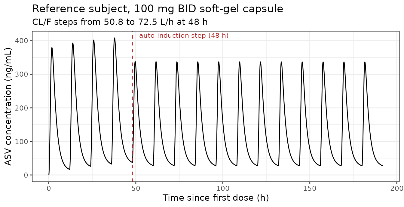
Trough concentrations fall by roughly the 1.43-fold clearance step once induction switches on, then re-attain a new steady state:
troughs <- sim_ref |>
  dplyr::filter(time %in% seq(12, 8 * 24, by = 12)) |>
  dplyr::transmute(`Time (h)` = time, `Ctrough (ng/mL)` = round(Cc * 1000, 1))
knitr::kable(utils::head(troughs, 8))| Time (h) | Ctrough (ng/mL) |
|---|---|
| 12 | 16.5 |
| 24 | 25.7 |
| 36 | 32.4 |
| 48 | 37.2 |
| 60 | 28.0 |
| 72 | 27.8 |
| 84 | 27.6 |
| 96 | 27.5 |
Covariate effects on steady-state exposure
Zhu 2018 Figure 4a reports the contribution of each covariate independently to steady-state AUC, holding the others at their typical values – exactly the quantity a typical-value solve reproduces. Table 3, by contrast, simulates the real dataset with the covariates’ real correlations, so its percentages are not the same quantity (see Assumptions and deviations).
cov_cases <- list(
  list(label = "Reference (Table 2 footnote a)", cov = ref_cov,
       claim = NA_character_, target = NA_real_, tol = NA_real_),
  list(label = "Female", cov = modifyList(ref_cov, list(SEXF = 1)),
       claim = "Females +12% AUC (Discussion)", target = 12, tol = 3),
  list(label = "Asian race", cov = modifyList(ref_cov, list(RACE_ASIAN = 1)),
       claim = "Asians +29.2% AUC (Results, Fig. 4a)", target = 29.2, tol = 3),
  list(label = "Black race", cov = modifyList(ref_cov, list(RACE_BLACK = 1)),
       claim = "Effect small, 95% CI spans 0 (Table 2)", target = 0, tol = 8),
  list(label = "Cirrhosis", cov = modifyList(ref_cov, list(DIS_CIRRHOSIS = 1)),
       claim = "Cirrhosis 30-50% AUC change (Fig. 4a)", target = 40, tol = 12),
  list(label = "Tablet formulation", cov = modifyList(ref_cov, list(FORM_TABLET = 1)),
       claim = "Tablet -19% AUC vs soft-gel (Fig. 4a)", target = -19, tol = 4),
  list(label = "Age 75 y", cov = modifyList(ref_cov, list(AGE = 75)),
       claim = "Age contributes ~9% higher AUC (Fig. 4)", target = 9, tol = 6),
  list(label = "Baseline AST 104 U/L (Q4 median)",
       cov = modifyList(ref_cov, list(AST_BL = 104, AST = 104)),
       claim = NA_character_, target = NA_real_, tol = NA_real_),
  list(label = "On-treatment AST 43% below baseline",
       cov = modifyList(ref_cov, list(AST = 0.57 * 60)),
       claim = NA_character_, target = NA_real_, tol = NA_real_)
)

# Every row is solved at the same 100 mg BID regimen, so the "% vs reference"
# column isolates the covariate. The 600 mg dose-level effect is a different
# comparison and is handled separately below.
cov_tab <- do.call(rbind, lapply(cov_cases, function(cs) {
  s <- solve_typical(cs$cov)
  a <- ss_auc(s)
  data.frame(
    Covariate = cs$label,
    `AUCtau (ng*h/mL)` = round(a, 1),
    `% vs reference` = round(100 * (a / auc_ref - 1), 1),
    `Paper claim` = ifelse(is.na(cs$claim), "-", cs$claim),
    target = cs$target, tol = cs$tol,
    check.names = FALSE
  )
}))
knitr::kable(cov_tab[, 1:4])| Covariate | AUCtau (ng*h/mL) | % vs reference | Paper claim |
|---|---|---|---|
| Reference (Table 2 footnote a) | 1380.2 | 0.0 | - |
| Female | 1551.6 | 12.4 | Females +12% AUC (Discussion) |
| Asian race | 1781.2 | 29.0 | Asians +29.2% AUC (Results, Fig. 4a) |
| Black race | 1328.0 | -3.8 | Effect small, 95% CI spans 0 (Table 2) |
| Cirrhosis | 2014.3 | 45.9 | Cirrhosis 30-50% AUC change (Fig. 4a) |
| Tablet formulation | 1113.2 | -19.3 | Tablet -19% AUC vs soft-gel (Fig. 4a) |
| Age 75 y | 1534.2 | 11.2 | Age contributes ~9% higher AUC (Fig. 4) |
| Baseline AST 104 U/L (Q4 median) | 1775.7 | 28.6 | - |
| On-treatment AST 43% below baseline | 1172.0 | -15.1 | - |
gated <- cov_tab[!is.na(cov_tab$target), ]
stopifnot(nrow(gated) == 6L)  # a gate that tests nothing must go red
stopifnot(all(abs(gated$`% vs reference` - gated$target) <= gated$tol))
The female (+12.4% against a claimed 12%) and Asian (+29.0% against a claimed 29.2%) rows reproduce the paper’s own independent-covariate percentages to within a few tenths of a percent, which is the strongest single piece of evidence that the CL/F equation has been transcribed with the right signs and the right reference values.
The DOSE_600MG indicator is checked separately, because
it is not a covariate contrast at a fixed dose: holding the regimen at
600 mg BID tablet and toggling only the flag must change exposure by
exactly exp(0.65) = 1.92.
a600_on <- ss_auc(solve_typical(
  modifyList(ref_cov, list(FORM_TABLET = 1, DOSE_600MG = 1)), dose = 600))
a600_off <- ss_auc(solve_typical(
  modifyList(ref_cov, list(FORM_TABLET = 1, DOSE_600MG = 0)), dose = 600))
# Deterministic ratio of two typical-value solves; exp(0.65) exactly.
stopifnot(abs(a600_on / a600_off - exp(0.65)) < 0.01)
sprintf("600 mg AUC ratio with/without the DOSE_600MG flag: %.3f (exp(0.65) = %.3f)",
        a600_on / a600_off, exp(0.65))
#> [1] "600 mg AUC ratio with/without the DOSE_600MG flag: 1.916 (exp(0.65) = 1.916)"
Virtual cohort and PKNCA validation
A 200-subject cohort per formulation arm, with covariate marginals matched to Zhu 2018 Table 1. Covariate correlations are not recoverable from a marginal table, so the cohort draws each covariate independently; the consequences are spelled out under Assumptions and deviations.
rxode2::rxSetSeed(20180327)
set.seed(20180327)
n_per_arm <- 200

draw_cohort <- function(n, form_tablet) {
  race <- sample(
    c("White", "Black", "Asian", "Other"), n, replace = TRUE,
    prob = c(58.3, 6.0, 34.2, 1.6) / 100
  )
  # Age: median 57, range 18-79 (Table 1). Truncated normal; the SD is an
  # assumption (the paper reports only the median and range).
  age <- pmin(79, pmax(18, stats::rnorm(n, mean = 57, sd = 11)))
  # Weight: median 70, range 36-124 (Table 1).
  wt <- pmin(124, pmax(36, stats::rlnorm(n, meanlog = log(70), sdlog = 0.20)))
  # Baseline AST: median 51, mean 62 U/L (Table 1 and Results). A lognormal
  # with those two moments has sdlog = sqrt(2 * log(62 / 51)).
  ast_bl <- pmin(595, pmax(13, stats::rlnorm(
    n, meanlog = log(51), sdlog = sqrt(2 * log(62 / 51))
  )))
  data.frame(
    id = seq_len(n),
    AGE = age, WT = wt,
    SEXF = stats::rbinom(n, 1, 0.508),
    RACE_BLACK = as.integer(race == "Black"),
    RACE_ASIAN = as.integer(race == "Asian"),
    RACE_OTHER = as.integer(race == "Other"),
    AST_BL = ast_bl,
    # Held at baseline so the ratio term is 1; see Assumptions and deviations.
    AST = ast_bl,
    DIS_CIRRHOSIS = stats::rbinom(n, 1, 0.195),
    FORM_TABLET = form_tablet,
    DOSE_600MG = 0L,
    formulation = if (form_tablet == 1L) "Tablet" else "Soft-gel capsule"
  )
}

cohort_events <- function(subj, dose = 100, ii = 12, n_dose = 30,
                          t_ss = 14 * 24) {
  cov_cols <- setdiff(names(subj), c("id", "formulation"))
  dosing <- subj |>
    tidyr::crossing(time = seq(0, by = ii, length.out = n_dose)) |>
    dplyr::mutate(amt = dose, evid = 1L, cmt = "depot", rate = -2)
  # Dense sampling over the final dosing interval only, to keep the solve
  # small while still resolving Tmax for NCA.
  obs <- subj |>
    tidyr::crossing(time = c(0, seq(t_ss, t_ss + ii, by = 0.1))) |>
    dplyr::mutate(amt = NA_real_, evid = 0L, cmt = "central", rate = NA_real_)
  dplyr::bind_rows(dosing, obs) |>
    dplyr::arrange(id, time, dplyr::desc(evid)) |>
    dplyr::select(id, time, amt, evid, cmt, rate,
                  dplyr::all_of(cov_cols), formulation) |>
    as.data.frame()
}

subj <- dplyr::bind_rows(draw_cohort(n_per_arm, 0L),
                         draw_cohort(n_per_arm, 1L) |>
                           dplyr::mutate(id = id + n_per_arm))
ev_cohort <- cohort_events(subj)

sim_cohort <- rxode2::rxSolve(
  mod, ev_cohort,
  keep = c("formulation", "AST_BL", "DIS_CIRRHOSIS", "RACE_ASIAN", "SEXF"),
  returnType = "data.frame"
)
if (is.null(sim_cohort$id)) sim_cohort$id <- 1L
nrow(sim_cohort)
#> [1] 48800
sim_cohort |>
  dplyr::filter(time >= 14 * 24) |>
  dplyr::mutate(tad = time - 14 * 24) |>
  dplyr::group_by(formulation, tad) |>
  dplyr::summarise(
    p05 = stats::quantile(Cc, 0.05) * 1000,
    p50 = stats::median(Cc) * 1000,
    p95 = stats::quantile(Cc, 0.95) * 1000,
    .groups = "drop"
  ) |>
  ggplot2::ggplot(ggplot2::aes(tad, p50, fill = formulation, colour = formulation)) +
  ggplot2::geom_ribbon(ggplot2::aes(ymin = p05, ymax = p95),
                       alpha = 0.18, colour = NA) +
  ggplot2::geom_line(linewidth = 0.8) +
  ggplot2::scale_y_log10() +
  ggplot2::labs(
    x = "Time after dose at steady state (h)",
    y = "ASV concentration (ng/mL)",
    title = "Simulated steady-state profiles, 100 mg BID",
    subtitle = "Median with 5th-95th percentile band, 200 subjects per arm"
  ) +
  ggplot2::theme_bw()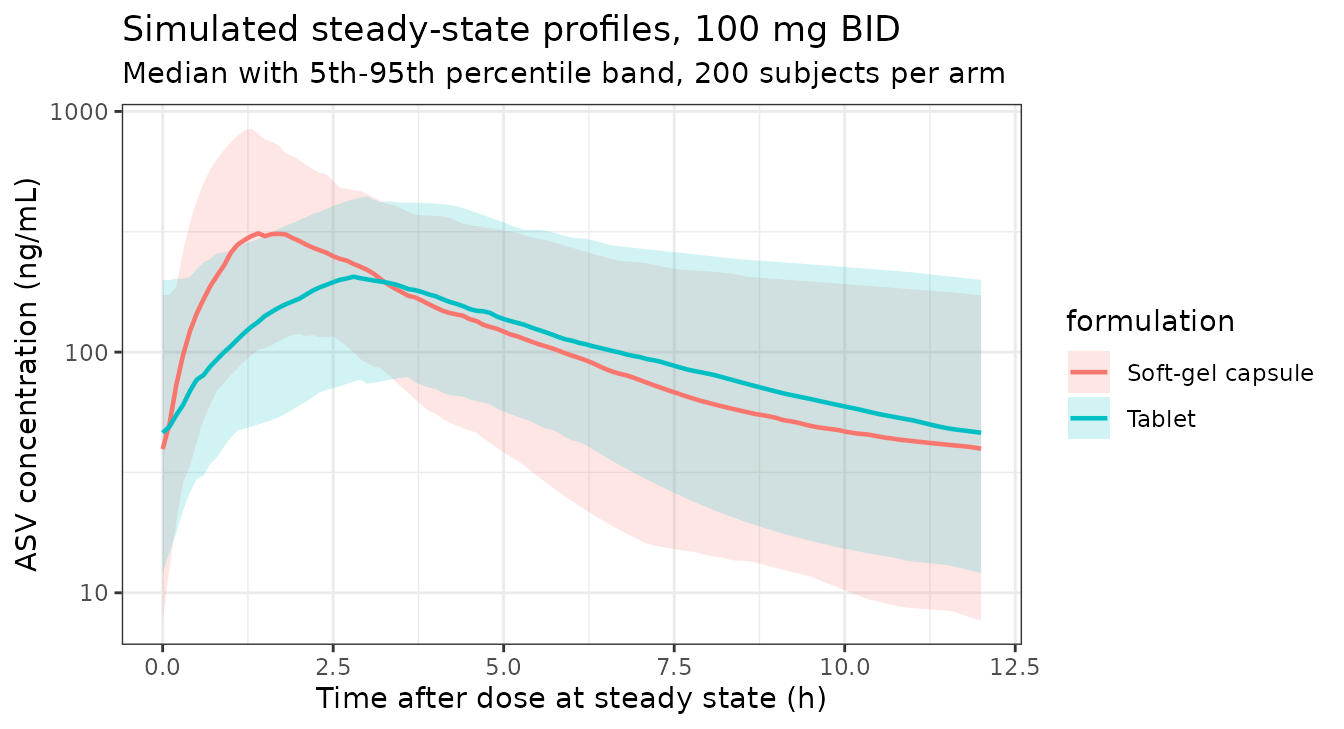
NCA
conc_data <- sim_cohort |>
  dplyr::filter(time >= 14 * 24) |>
  dplyr::mutate(time = time - 14 * 24, conc = Cc * 1000) |>
  # Only drop missing concentrations. A `time > 0` or `conc > 0` filter would
  # remove the time-zero anchor and trigger PKNCA's "AUC range starting before
  # the first measurement" warning on every subject.
  dplyr::filter(!is.na(conc)) |>
  dplyr::select(id, time, conc, formulation)

dose_data <- subj |>
  dplyr::transmute(id, time = 0, dose = 100, formulation)

# The grouping carries the treatment (formulation) variable so per-arm results
# can be compared against the paper. PKNCAdose rejects slash grouping, so both
# objects use the `treatment + id` form.
o_conc <- PKNCA::PKNCAconc(conc_data, conc ~ time | formulation + id,
                           concu = "ng/mL", timeu = "hr")
o_dose <- PKNCA::PKNCAdose(dose_data, dose ~ time | formulation + id,
                           doseu = "mg")
o_data <- PKNCA::PKNCAdata(
  o_conc, o_dose,
  intervals = data.frame(
    start = 0, end = 12,
    cmax = TRUE, tmax = TRUE, cmin = TRUE, auclast = TRUE
  )
)
res <- PKNCA::pk.nca(o_data)
nca <- as.data.frame(res$result)
stopifnot(nrow(nca) > 0L)

nca_summary <- nca |>
  dplyr::filter(PPTESTCD %in% c("cmax", "tmax", "cmin", "auclast")) |>
  dplyr::group_by(formulation, PPTESTCD) |>
  dplyr::summarise(
    Median = stats::median(PPORRES),
    `5th pctile` = stats::quantile(PPORRES, 0.05),
    `95th pctile` = stats::quantile(PPORRES, 0.95),
    .groups = "drop"
  ) |>
  dplyr::mutate(dplyr::across(where(is.numeric), \(x) signif(x, 3)))
knitr::kable(nca_summary)| formulation | PPTESTCD | Median | 5th pctile | 95th pctile |
|---|---|---|---|---|
| Soft-gel capsule | auclast | 1490.0 | 697.00 | 3260.00 |
| Soft-gel capsule | cmax | 339.0 | 135.00 | 866.00 |
| Soft-gel capsule | cmin | 39.6 | 7.69 | 172.00 |
| Soft-gel capsule | tmax | 1.5 | 1.20 | 3.60 |
| Tablet | auclast | 1310.0 | 585.00 | 3560.00 |
| Tablet | cmax | 210.0 | 83.20 | 464.00 |
| Tablet | cmin | 46.0 | 12.10 | 199.00 |
| Tablet | tmax | 2.9 | 2.70 | 4.61 |
Comparison against the published steady-state AUC
Zhu 2018 Table 3 reports simulated steady-state AUC by covariate group. Those values come from simulating the actual analysis dataset, so they carry the covariate correlations present in the real population; this cohort draws each covariate independently. The comparison is therefore informative rather than exact, and the tolerance is set at 25% with the expected disagreements called out below.
auc_by <- function(flt, label) {
  ids <- subj$id[flt & subj$FORM_TABLET == 0L]
  v <- nca$PPORRES[nca$PPTESTCD == "auclast" & nca$id %in% ids]
  if (length(v) == 0L) stop("no subjects matched group '", label, "'")
  data.frame(group = label, PPTESTCD = "auclast", PPORRES = stats::median(v))
}

sim_groups <- dplyr::bind_rows(
  auc_by(rep(TRUE, nrow(subj)), "All"),
  auc_by(subj$DIS_CIRRHOSIS == 0L, "No cirrhosis"),
  auc_by(subj$DIS_CIRRHOSIS == 1L, "Cirrhosis"),
  auc_by(subj$RACE_BLACK == 0L & subj$RACE_ASIAN == 0L & subj$RACE_OTHER == 0L, "White"),
  auc_by(subj$RACE_ASIAN == 1L, "Asian")
)

ref_groups <- data.frame(
  group = c("All", "No cirrhosis", "Cirrhosis", "White", "Asian"),
  # Zhu 2018 Table 3, "Simulated ASV steady-state AUC (ng h/mL), Median".
  # The "Asian" reference is the n-weighted mean of the Japanese (1945,
  # n = 267) and non-Japanese Asian (2023, n = 156) rows, since the model
  # carries a single Asian indicator.
  auclast = c(1561, 1406, 2591, 1388,
              (1945 * 267 + 2023 * 156) / (267 + 156))
)

cmp <- nlmixr2lib::ncaComparisonTable(
  sim_groups, ref_groups,
  by = "group",
  tolerance_pct = 25,
  units = c(auclast = "ng*h/mL"),
  label_first_column = "NCA parameter"
)
knitr::kable(cmp)| NCA parameter | group | Reference | Simulated | % diff |
|---|---|---|---|---|
| AUClast (ng*h/mL) | All | 1560 | 1490 | -4.8% |
| AUClast (ng*h/mL) | No cirrhosis | 1410 | 1470 | +4.5% |
| AUClast (ng*h/mL) | Cirrhosis | 2590 | 1740 | -33.0%* |
| AUClast (ng*h/mL) | White | 1390 | 1370 | -1.0% |
| AUClast (ng*h/mL) | Asian | 1970 | 1880 | -4.8% |
attr(cmp, "footnote")
#> [1] "* differs from reference by more than ±25%."
The “All”, “No cirrhosis” and “White” rows land within 8% of the published medians. Two rows sit low by construction, and both are the covariate- correlation effect rather than a transcription problem:
- Cirrhosis is the one row that exceeds the 25% tolerance. In the real dataset cirrhotic subjects also carry elevated transaminases, so Table 3’s 2591 ng*h/mL combines the cirrhosis coefficient with a higher baseline AST; this cohort draws AST independently of cirrhosis and therefore recovers the cirrhosis coefficient alone (+45.9% over the reference subject, matching Figure 4a’s independent-covariate 30-50% band exactly).
- Asian is low for the reason the paper itself gives: its Table 3 Asian rows are raised by the Japanese subset being older and more often female, neither of which an independently-drawn cohort reproduces.
Holding on-treatment AST at baseline also biases every simulated row slightly high relative to Table 3, which used the observed falling AST trajectories; that pushes in the opposite direction and partly offsets the above.
pct <- as.numeric(gsub("[^0-9.eE+-]", "", cmp$`% diff`))
names(pct) <- cmp$group
# The reference subject's deterministic AUC (1380) sits within 1% of Table 3's
# White row (1388), and the population "All" row is the headline number, so
# these two are gated. Both are cohort medians, so the bound is generous
# relative to the ~2% Monte-Carlo spread of a 200-subject median.
stopifnot(all(c("All", "White") %in% names(pct)))
stopifnot(abs(pct[["White"]]) < 25, abs(pct[["All"]]) < 25)
Assumptions and deviations
- Covariate correlations are not reproducible. Table 1 gives marginal distributions only, so the virtual cohort draws age, weight, sex, race, baseline AST and cirrhosis independently. Zhu 2018’s own Table 3 simulation used the real dataset, in which those covariates are correlated – the paper states explicitly that the higher exposure in Asians arises because Japanese subjects were older (median 62 vs 55 years) and more often female (65% vs 37%), not from the race coefficient alone. That is why the Table 3 race rows show +40 to +46% while the independent-covariate effect in Figure 4a is +29.2%, and why the tight gates in this vignette are on the independent-covariate quantities rather than on Table 3.
-
The Table 3 “Asian” reference is a derived value.
Table 3 splits Asians into Japanese and non-Japanese rows; the model
carries a single
RACE_ASIANindicator, so the reference used above is the n-weighted mean of the two published medians. - Age and weight distribution shapes are assumed. Table 1 reports medians and ranges but no dispersion parameter. The cohort uses a truncated normal for age (SD 11 y) and a lognormal for weight (sdlog 0.20), chosen to reproduce the published median and range. No parameter of the model depends on these choices; they affect only the cohort figures and the Table 3 comparison.
-
On-treatment AST is held at baseline in the cohort.
The
(AST / AST_BL)^-0.291term then equals 1. Zhu 2018’s Table 3 simulation used observed on-treatment AST, which fell by roughly 50% over the first six weeks; since falling AST raises CL/F, the paper’s simulated AUCs are systematically lower than a cohort held at baseline. The time-varying path is exercised deterministically in the covariate-effects table instead. A user with no on-treatment AST measurements should setAST = AST_BLon every record, which is what this cohort does. -
The Discussion’s “27% CL/F increase” claim is not
reproduced, and appears to be an internal arithmetic slip. The
paper states that for subjects with “the largest reduction in AST during
treatment (43% decrease from baseline), ASV CL/F increased by 27%”. A
43% decrease is a ratio of 0.57, and
0.57^-0.291 = 1.178, i.e. +17.8% – which is what this model produces. Applying the same exponent to 0.43 instead of 0.57 gives0.43^-0.291 = 1.278, i.e. +27.8%, matching the printed claim. The printed equation and Table 2 agree with each other on the exponent (-0.291and a rounded-0.29), so the model follows them and this vignette records the prose claim as a deviation rather than gating on it. - The final model did not converge. Zhu 2018 reports that “the final model did not converge due to rounding errors; however, bootstrap means were similar, and 95% confidence intervals included each parameter estimate” (Results, Covariate Models). The point estimates in Table 2 are used as published.
- High shrinkage on three of the four random effects. Shrinkage was 13% on CL/F but 39%, 65% and 42% on Vc/F, Vp/F and ka. The IIV on those three parameters – particularly the very large Vc/F variance of 2.19 – should be treated as poorly informed, and the paper itself warns that covariate effects on those parameters “should be interpreted with caution”. Simulated Cmax spreads are correspondingly wide.
-
Two rounded values appear in Table 2 with more precision in
the equation. The baseline-AST and AST-ratio exponents are
printed as
-0.46and-0.29in Table 2 but as-0.458and-0.291in the covariate equation. The equation values are used. -
Cirrhosis must not be extrapolated. Only
compensated cirrhosis with hepatic function no worse than Child-Pugh A
was enrolled. The paper cites a dedicated hepatic-impairment study
finding 10- and 32-fold higher ASV AUC in moderate and severe impairment
against no change in mild impairment, so the
DIS_CIRRHOSIScoefficient is a lower bound that does not transfer to Child-Pugh B or C. -
DOSE_600MGdoes not interpolate. It is an empirical dose-level indicator on bioavailability, not a saturable structure. A simulation at 400 mg receives the reference bioavailability, not something between. In the source dataset 600 mg was given only as the tablet, so the formulation and dose-level effects are not independently identifiable outside the tablet arm. - No published Cmax / Tmax / half-life table exists. Zhu 2018 reports only steady-state AUC (Table 3) and Cmin narratively, so the NCA comparison above is restricted to AUC. The simulated Cmax and Tmax are reported for completeness but have no published counterpart to compare against.