Nivolumab and ipilimumab pediatric population PK (Hu 2024)
Source:vignettes/articles/Hu_2024_nivolumab_ipilimumab_pediatric.Rmd
Hu_2024_nivolumab_ipilimumab_pediatric.RmdModel and source
Hu 2024 developed two independent pooled adult-plus-pediatric population PK models – one for nivolumab, one for ipilimumab – to answer a single question: after body size has been accounted for, is there anything left of the pediatric-versus-adult difference in monoclonal-antibody PK? The answer the paper reaches is yes, and that the residual effect is tumour-type dependent. Because the authors fitted the two drugs separately, on different datasets and with different structural forms (nivolumab time-varying clearance, ipilimumab stationary clearance), the extraction is two model files sharing this one vignette.
nivo <- rxode2::rxode(readModelDb("Hu_2024_nivolumab"))
#> ℹ parameter labels from comments will be replaced by 'label()'
ipi  <- rxode2::rxode(readModelDb("Hu_2024_ipilimumab"))
#> ℹ parameter labels from comments will be replaced by 'label()'- Citation: Hu Z, Liu S, Zhao Y, Du S, Hamuro L, Shen J, Roy A, Zhu L. Nivolumab and ipilimumab population pharmacokinetics in support of pediatric dose recommendations-Going beyond the body-size effect. CPT Pharmacometrics Syst Pharmacol. 2024;13(3):476-493. doi:10.1002/psp4.13098
- Nivolumab model: Two-compartment population PK model with time-varying clearance for intravenous nivolumab (anti-PD-1 IgG4) in a pooled adult and pediatric (1-17 years) oncology population, with tumor-type-dependent pediatric effects on baseline clearance beyond body size (Hu 2024)
- Ipilimumab model: Two-compartment population PK model with stationary clearance for intravenous ipilimumab (anti-CTLA-4 IgG1) in a pooled adult and pediatric (1-17 years) oncology population, with tumor-type-dependent pediatric effects on clearance beyond body size (Hu 2024)
- Article: https://doi.org/10.1002/psp4.13098
- Supplement (Appendix S1 supplementary results and tables, Appendix File S2 and S3 NONMEM control streams): https://europepmc.org/article/PMC/PMC10941504
Population
Nivolumab (Table 1). 13,104 concentrations from 2,325 patients across 13 studies, of whom 275 were pediatric. The analysis populations are adult melanoma (n = 993, the reference), adult lymphoma (n = 274), adult glioblastoma (n = 556), adult other solid tumours (n = 227), pediatric solid tumours (n = 79), pediatric lymphoma (n = 46), and pediatric CNS tumours (n = 150). Overall age median 55 years (range 1-90), baseline body weight median 76.2 kg (range 9.3-168), 36.5% female, 90.3% White. The pediatric cohorts are markedly smaller in both weight and lean body mass than the adults: pediatric CNS-tumour median weight 33 kg with mean lean body mass 30.2 kg, against an adult-melanoma mean weight of 82.3 kg and mean lean body mass of 57.7 kg.
Ipilimumab (Table 2). 6,020 concentrations from 1,427 patients across 10 studies, of whom 138 were pediatric: adult melanoma (n = 1261, the reference), adult CNS tumours (n = 6), adult other solid tumours (n = 22), pediatric solid tumours (n = 43), pediatric CNS tumours (n = 72), and pediatric melanoma (n = 23). Overall age median 58 years (range 1-89), weight median 78.1 kg (range 10.2-160), 36.9% female, 94.8% White.
Both analyses estimated lean body mass by the Boer equation in adults and the Peter equation in children (Table 1 Note).
The same information is available programmatically from each model’s
population metadata:
str(nivo$population, max.level = 1, give.attr = FALSE)
#> List of 18
#>  $ species           : chr "human"
#>  $ n_subjects        : int 2325
#>  $ n_studies         : int 13
#>  $ n_observations    : int 13104
#>  $ n_pediatric       : int 275
#>  $ age_range         : chr "1-90 years (pediatric 1-17 years; adult >= 18 years)"
#>  $ age_median        : chr "55 years overall; pediatric solid tumors 12 y, pediatric lymphoma 15 y, pediatric CNS tumors 10 y"
#>  $ weight_range      : chr "9.3-168 kg"
#>  $ weight_median     : chr "76.2 kg overall; pediatric solid tumors 43.2 kg, pediatric lymphoma 58.2 kg, pediatric CNS tumors 33 kg"
#>  $ sex_female_pct    : num 36.5
#>  $ race_ethnicity    : Named num [1:4] 90.3 2.8 3.7 3.2
#>  $ disease_state     : chr "Advanced melanoma (n = 994), Hodgkin / non-Hodgkin lymphoma (n = 320), central nervous system tumors including "| __truncated__
#>  $ dose_range        : chr "Nivolumab 0.1-20 mg/kg or 240/480 mg flat intravenous infusion q2w, q3w, or q4w, alone or combined with ipilimu"| __truncated__
#>  $ regions           : chr "Pooled global phase I, I/II, II, and III studies (13 trials; Table S1)"
#>  $ performance_status: chr "ECOG PS 0 50.5%, PS 1 45.1%, PS 2 4.3%, PS 3 0.04%"
#>  $ renal_function    : chr "Baseline eGFR mean 93.8 (SD 22.8) mL/min/1.73 m^2, median 92.9"
#>  $ body_composition  : chr "Baseline lean body mass mean 54.5 (SD 13.8) kg, median 55.8 kg; estimated by the Boer equation (adults) and the"| __truncated__
#>  $ notes             : chr "Baseline demographics per Hu 2024 Table 1 (N = 2325 across 13 nivolumab studies, of whom 275 were pediatric). T"| __truncated__
Source trace
Every ini() entry in both model files carries an in-file
comment naming its source location. The table below collects them.
| Equation / parameter | Value | Source location |
|---|---|---|
CL_i(t) = CL0TV_i * exp(Emax_i * t^HILL / (T50^HILL + t^HILL)) * exp(eta_CL) |
n/a | Hu 2024 Results, first nivolumab equation |
CL0TV_i = CL0REF * (WTB/75)^CLWTB * (eGFR/90)^CLeGFR * exp(...) |
n/a | Hu 2024 Results, nivolumab CL0TV,i equation |
EMAX_i = EMAXREF + EMAXPS + EMAXCOMBO + EMAXHL + EMAXOTH + EMAXpedCNST + eta_EMAX |
n/a | Hu 2024 Results, nivolumab EMAX_i equation |
VC_i = VCREF * (LBM/55)^VCLBM * exp(VCSEX) * exp(VCado) * exp(VCped) * exp(eta_VC) |
n/a | Hu 2024 Results, nivolumab VC_i equation |
Q_i = QREF * (WTB/75)^QWTB * exp(eta_Q);
VP_i = VPREF * (LBM/55)^VPLBM * exp(eta_VP)
|
n/a | Hu 2024 Results, nivolumab Q_i and VP_i
equations |
nivolumab CL0REF
|
9.66 mL/h | Table 4 |
nivolumab VCREF, QREF,
VPREF
|
4.01 L, 35.9 mL/h, 2.77 L | Table 4 |
nivolumab CLWTB, CLeGFR,
VCLBM
|
0.630, 0.0982, 0.932 | Table 4 |
nivolumab CLSEX, CLPS,
CLRAAA, CLRAAS
|
-0.0998, 0.166, 0.0693, 0.00333 | Table 4 |
nivolumab EMAXREF, T50,
HILL
|
-0.298, 2670 h, 2.32 | Table 4 |
nivolumab CLHL, CLGBM,
CLOTH
|
-0.382, -0.578, 0.00699 | Table 4 |
nivolumab CLPEDST, CLADOST,
CLPEDHL, CLPEDCNST
|
-0.580, -0.223, -0.411, -0.801 | Table 4 |
nivolumab CLI1Q3, CLI3Q3,
CLBVCO
|
0.0973, 0.349, 0.132 | Table 4 |
nivolumab EMAXPS, EMAXIPICO,
EMAXHL, EMAXOTH, EMAXPEDCNST
|
-0.157, -0.124, 0.132, 0.118, 0.696 | Table 4 |
nivolumab VCSEX, VCPED,
VCADO
|
0.0195, -0.277, -0.273 | Table 4 |
| nivolumab omega^2 CL / VC / covariance / Emax | 0.108, 0.0751, 0.0220, 0.160 | Table 4 |
| nivolumab omega^2 Q / VP / covariance | constrained equal to the CL / VC block | Appendix File S2, $OMEGA BLOCK(2) SAME
|
| nivolumab proportional residual error | 0.199 | Table 4 |
QWTB = CLWTB, VPLBM = VCLBM
|
0.630, 0.932 | Figure 1 caption (“fixed to be similar to those of CL and VC”) |
| adult-CNS-tumour Emax = 0 (stationary CL) | n/a | Appendix File S2, IF (POP_I .EQ. 4) EMAX = 0
|
| pediatric ST / HL Emax offsets = 0 | n/a | Methods; Appendix File S2 THETA(38) and
THETA(39) = 0 FIX
|
CL_i = CL0TV_i * exp(eta_CL) (ipilimumab,
stationary) |
n/a | Hu 2024 Results, first ipilimumab equation |
CL0TV_i = CL0REF * (LBM/55)^CLLBM * exp(...) |
n/a | Hu 2024 Results, ipilimumab CL0TV,i equation (see
Errata on the printed subscript) |
VC_i = VCREF * (LBM/55)^VCLBM * exp(VCado) * exp(VCped) * exp(eta_VC) |
n/a | Hu 2024 Results, ipilimumab VC_i equation |
ipilimumab CLREF, VCREF,
QREF, VPREF
|
13.5 mL/h, 3.90 L, 35.8 mL/h, 3.47 L | Table 5 |
ipilimumab CLLBM, VCLBM
|
0.789, 0.874 | Table 5 |
ipilimumab CLCNST, CLOTH,
CLPEDOTH, CLPEDCNST,
CLPEDMEL
|
-0.661, -0.698, -0.462, -0.668, -0.347 | Table 5 |
ipilimumab CLN1Q3, CLN3Q3
|
0.0417, 0.316 | Table 5 |
ipilimumab VCPED, VCADO
|
-0.296, -0.217 | Table 5 |
| ipilimumab omega^2 CL / VC / covariance | 0.147, 0.0531, 0.0258 | Table 5 |
| ipilimumab residual error (proportional, additive) | 0.185, 1.14 ug/mL | Table 5 |
age bands < 12, 12-17,
>= 18 years |
n/a | Methods; Appendix Files S2 and S3 (AGE <= 11,
12 <= AGE <= 17) |
Structural verification of the covariate wiring
The paper reports every patient-population effect twice: once as a
coefficient in Table 4 / Table 5, and once as a percentage change in the
Results narrative. Because those percentages are exactly
exp(theta), reproducing them from a typical-value solve is
a direct check that each coefficient reaches the correct (tumour type x
age band) cell of the model – the one thing a transcription of this
model can most easily get wrong.
# Reference covariates from Hu 2024 Table 4 Note / Results: 75 kg, LBM 55 kg,
# eGFR 90 mL/min/1.73 m^2, male, White/Other, performance status 0, monotherapy.
nivo_cells <- tibble::tribble(
  ~cell,                                   ~AGE, ~TUMTP_LYMPH, ~TUMTP_CNS_PRIM, ~TUMTP_OTHER,
  "Adult melanoma (reference)",              55,            0,               0,            0,
  "Adult lymphoma",                          36,            1,               0,            0,
  "Adult CNS tumour (glioblastoma)",         57,            0,               1,            0,
  "Adult other solid tumour",                62,            0,               0,            1,
  "Adolescent (12-17 y) solid tumour",       15,            0,               0,            1,
  "Young pediatric (<12 y) solid tumour",     8,            0,               0,            1,
  "Pediatric (<18 y) lymphoma",              15,            1,               0,            0,
  "Pediatric (<18 y) CNS tumour",            10,            0,               1,            0
) |>
  mutate(
    id = row_number(), WT = 75, LBM = 55, CRCL = 90, SEXF = 0,
    ECOG_GE1 = 0, RACE_BLACK = 0, RACE_ASIAN = 0,
    CONMED_IPI_1Q3W = 0, CONMED_IPI_3Q3W = 0,
    CONMED_BRENTUXIMAB = 0, CONMED_IPI_ANY = 0
  )

# One dose plus a t = 0 observation. At t = 0 the sigmoid time term is exactly
# zero, so the returned `cl` is the baseline CL0 the paper tabulates.
nivo_cell_ev <- bind_rows(
  nivo_cells |> mutate(time = 0, amt = 240, evid = 1L, cmt = "central"),
  nivo_cells |> mutate(time = 0, amt = NA_real_, evid = 0L, cmt = "central")
) |>
  arrange(id, desc(evid))

nivo_cell_sim <- rxode2::rxSolve(
  rxode2::zeroRe(nivo), events = nivo_cell_ev, keep = "cell"
) |>
  as.data.frame() |>
  group_by(cell) |>
  summarise(cl = first(cl), vc = first(vc), .groups = "drop")
#> ℹ omega/sigma items treated as zero: 'etalcl', 'etalvc', 'etalq', 'etalvp', 'etacl_time_max'
#> Warning: multi-subject simulation without without 'omega'

nivo_ref <- nivo_cell_sim$cl[nivo_cell_sim$cell == "Adult melanoma (reference)"]
nivo_ref_vc <- nivo_cell_sim$vc[nivo_cell_sim$cell == "Adult melanoma (reference)"]
nivo_expected <- tibble::tribble(
  ~cell,                                   ~theta,   ~published_pct_lower,
  "Adult melanoma (reference)",             0,       0,
  "Adult lymphoma",                        -0.382,  32,
  "Adult CNS tumour (glioblastoma)",       -0.578,  44,
  "Adult other solid tumour",               0.00699, 0,
  "Adolescent (12-17 y) solid tumour",     -0.223,  20,
  "Young pediatric (<12 y) solid tumour",  -0.580,  44,
  "Pediatric (<18 y) lymphoma",            -0.411,  34,
  "Pediatric (<18 y) CNS tumour",          -0.801,  55
)

nivo_chk <- nivo_cell_sim |>
  left_join(nivo_expected, by = "cell") |>
  mutate(
    ratio_model    = cl / nivo_ref,
    ratio_expected = exp(theta),
    pct_lower      = 100 * (1 - ratio_model),
    abs_err        = abs(ratio_model - ratio_expected)
  )

# Deterministic (zeroRe) solve of a closed-form algebraic expression: the only
# error here is floating point, so the bound is tight on purpose.
stopifnot(max(nivo_chk$abs_err) < 1e-8)
# The narrative percentages in Hu 2024 Results are rounded to whole percent.
stopifnot(max(abs(nivo_chk$pct_lower - nivo_chk$published_pct_lower)) < 1)

nivo_chk |>
  select(cell, ratio_model, pct_lower, published_pct_lower) |>
  mutate(across(c(ratio_model, pct_lower), \(x) round(x, 3))) |>
  rename(
    "Patient population"                = cell,
    "CL0 / CL0 (adult MEL)"             = ratio_model,
    "% lower (model)"                   = pct_lower,
    "% lower (Hu 2024 Results)"         = published_pct_lower
  ) |>
  knitr::kable(
    caption = paste(
      "Nivolumab baseline-clearance covariate effects reproduced from the",
      "packaged model at the paper's reference covariates. Compare with the",
      "Hu 2024 Results narrative and Figure 1a."
    )
)| Patient population | CL0 / CL0 (adult MEL) | % lower (model) | % lower (Hu 2024 Results) |
|---|---|---|---|
| Adolescent (12-17 y) solid tumour | 0.800 | 19.989 | 20 |
| Adult CNS tumour (glioblastoma) | 0.561 | 43.898 | 44 |
| Adult lymphoma | 0.682 | 31.750 | 32 |
| Adult melanoma (reference) | 1.000 | 0.000 | 0 |
| Adult other solid tumour | 1.007 | -0.701 | 0 |
| Pediatric (<18 y) CNS tumour | 0.449 | 55.112 | 55 |
| Pediatric (<18 y) lymphoma | 0.663 | 33.701 | 34 |
| Young pediatric (<12 y) solid tumour | 0.560 | 44.010 | 44 |
The central-volume age effects are gated the same way. Hu 2024
reports both pediatric bands at 24% lower VC than
adults.
nivo_vc_chk <- nivo_cell_sim |>
  mutate(
    band = case_when(
      cell %in% c("Adolescent (12-17 y) solid tumour",
                  "Pediatric (<18 y) lymphoma")        ~ "Adolescent (12-17 y)",
      cell %in% c("Young pediatric (<12 y) solid tumour",
                  "Pediatric (<18 y) CNS tumour")      ~ "Young pediatric (<12 y)",
      TRUE                                              ~ "Adult"
    ),
    ratio_vc = vc / nivo_ref_vc
  ) |>
  group_by(band) |>
  summarise(ratio_vc = mean(ratio_vc), .groups = "drop")

vc_expected <- c(
  "Adult"                   = 1,
  "Adolescent (12-17 y)"    = exp(-0.273),
  "Young pediatric (<12 y)" = exp(-0.277)
)
stopifnot(max(abs(nivo_vc_chk$ratio_vc - vc_expected[nivo_vc_chk$band])) < 1e-8)
# Hu 2024 Results: "adolescent (12-17 years) and pediatric (<12 years) patients
# had 24% lower VC than adult patients".
stopifnot(all(abs(100 * (1 - nivo_vc_chk$ratio_vc[nivo_vc_chk$band != "Adult"]) - 24) < 1))

nivo_vc_chk |>
  mutate(`% lower than adult` = round(100 * (1 - ratio_vc), 1),
         ratio_vc = round(ratio_vc, 3)) |>
  rename("Age band" = band, "VC / VC (adult)" = ratio_vc) |>
knitr::kable(caption = "Nivolumab central-volume age effects (Hu 2024 Figure 1b).")| Age band | VC / VC (adult) | % lower than adult |
|---|---|---|
| Adolescent (12-17 y) | 0.761 | 23.9 |
| Adult | 1.000 | 0.0 |
| Young pediatric (<12 y) | 0.758 | 24.2 |
The same check for the ipilimumab model, whose patient-population
factor pools the whole under-18 range on CL (no 12-year
split) but does split VC at 12 years.
ipi_cells <- tibble::tribble(
  ~cell,                                 ~AGE, ~TUMTP_MEL, ~TUMTP_CNS_PRIM, ~TUMTP_OTHER, ~theta, ~published_pct_lower,
  "Adult melanoma (reference)",            55,          1,               0,            0,  0,      0,
  "Adult CNS tumour",                      19,          0,               1,            0, -0.661, 48,
  "Adult other solid tumour",              21,          0,               0,            1, -0.698, 50,
  "Pediatric (<18 y) other solid tumour",  13,          0,               0,            1, -0.462, 37,
  "Pediatric (<18 y) CNS tumour",          10,          0,               1,            0, -0.668, 49,
  "Pediatric (<18 y) melanoma",            13,          1,               0,            0, -0.347, 29
) |>
  mutate(id = row_number(), LBM = 55, CONMED_NIVO_1Q3W = 0, CONMED_NIVO_3Q3W = 0)

ipi_cell_ev <- bind_rows(
  ipi_cells |> mutate(time = 0, amt = 200, evid = 1L, cmt = "central"),
  ipi_cells |> mutate(time = 0, amt = NA_real_, evid = 0L, cmt = "central")
) |>
  select(-theta, -published_pct_lower) |>
  arrange(id, desc(evid))

ipi_cell_sim <- rxode2::rxSolve(
  rxode2::zeroRe(ipi), events = ipi_cell_ev, keep = "cell"
) |>
  as.data.frame() |>
  group_by(cell) |>
  summarise(cl = first(cl), vc = first(vc), .groups = "drop")
#> ℹ omega/sigma items treated as zero: 'etalcl', 'etalvc'
#> Warning: multi-subject simulation without without 'omega'

ipi_ref <- ipi_cell_sim$cl[ipi_cell_sim$cell == "Adult melanoma (reference)"]

ipi_chk <- ipi_cell_sim |>
  left_join(ipi_cells |> select(cell, theta, published_pct_lower), by = "cell") |>
  mutate(ratio_model = cl / ipi_ref,
         pct_lower   = 100 * (1 - ratio_model),
         abs_err     = abs(ratio_model - exp(theta)))

stopifnot(max(ipi_chk$abs_err) < 1e-8)
stopifnot(max(abs(ipi_chk$pct_lower - ipi_chk$published_pct_lower)) < 1)

ipi_chk |>
  select(cell, ratio_model, pct_lower, published_pct_lower) |>
  mutate(across(c(ratio_model, pct_lower), \(x) round(x, 3))) |>
  rename(
    "Patient population"        = cell,
    "CL / CL (adult MEL)"       = ratio_model,
    "% lower (model)"           = pct_lower,
    "% lower (Hu 2024 Results)" = published_pct_lower
  ) |>
  knitr::kable(
    caption = paste(
      "Ipilimumab clearance covariate effects reproduced from the packaged",
      "model at LBM = 55 kg. Compare with the Hu 2024 Results narrative and",
      "Figure 2."
    )
)| Patient population | CL / CL (adult MEL) | % lower (model) | % lower (Hu 2024 Results) |
|---|---|---|---|
| Adult CNS tumour | 0.516 | 48.367 | 48 |
| Adult melanoma (reference) | 1.000 | 0.000 | 0 |
| Adult other solid tumour | 0.498 | 50.242 | 50 |
| Pediatric (<18 y) CNS tumour | 0.513 | 48.727 | 49 |
| Pediatric (<18 y) melanoma | 0.707 | 29.319 | 29 |
| Pediatric (<18 y) other solid tumour | 0.630 | 36.998 | 37 |
The time-varying-clearance arm
Figure 1b of Hu 2024 reports the steady-state-to-baseline clearance
ratio and states the identity used to compute it:
CLss / CL0 = exp(EMAX). Simulating a typical subject far
past T50 recovers that ratio, and does so per covariate
cell – including the adult CNS-tumour cell, where the source control
stream sets EMAX to exactly zero so clearance is
stationary. That last row is not visible anywhere in the printed
equations; it comes from Appendix File S2.
emax_cells <- tibble::tribble(
  ~cell,                              ~AGE, ~TUMTP_LYMPH, ~TUMTP_CNS_PRIM, ~TUMTP_OTHER, ~ECOG_GE1, ~CONMED_IPI_ANY, ~emax_expected,
  "Adult MEL, mono, PS 0",              55,            0,               0,            0,         0,               0, -0.298,
  "Adult MEL, mono, PS > 0",            55,            0,               0,            0,         1,               0, -0.298 - 0.157,
  "Adult MEL + ipilimumab, PS 0",       55,            0,               0,            0,         0,               1, -0.298 - 0.124,
  "Adult lymphoma, mono, PS 0",         36,            1,               0,            0,         0,               0, -0.298 + 0.132,
  "Adult other ST, mono, PS 0",         62,            0,               0,            1,         0,               0, -0.298 + 0.118,
  "Pediatric CNS tumour, mono, PS 0",   10,            0,               1,            0,         0,               0, -0.298 + 0.696,
  "Adult CNS tumour (GBM), mono, PS 0", 57,            0,               1,            0,         0,               0,  0
) |>
  mutate(
    id = row_number(), WT = 75, LBM = 55, CRCL = 90, SEXF = 0,
    RACE_BLACK = 0, RACE_ASIAN = 0, CONMED_IPI_1Q3W = 0,
    CONMED_IPI_3Q3W = 0, CONMED_BRENTUXIMAB = 0
  )

# t = 0 gives CL0; t = 2000 days is ~18 x T50, so the sigmoid has reached
# 99.88% of its plateau. The residual approach error is < 0.1% and is the
# reason the tolerance below is 0.5% rather than machine epsilon.
emax_ev <- bind_rows(
  emax_cells |> mutate(time = 0, amt = 240, evid = 1L, cmt = "central"),
  tidyr::crossing(emax_cells, time = c(0, 2000)) |>
    mutate(amt = NA_real_, evid = 0L, cmt = "central")
) |>
  select(-emax_expected) |>
  arrange(id, time, desc(evid))

emax_sim <- rxode2::rxSolve(
  rxode2::zeroRe(nivo), events = emax_ev, keep = "cell"
) |>
  as.data.frame() |>
  group_by(cell) |>
  summarise(cl0 = cl[which.min(time)], clss = cl[which.max(time)], .groups = "drop") |>
  left_join(emax_cells |> select(cell, emax_expected), by = "cell") |>
  mutate(ratio_model = clss / cl0, ratio_expected = exp(emax_expected))
#> ℹ omega/sigma items treated as zero: 'etalcl', 'etalvc', 'etalq', 'etalvp', 'etacl_time_max'
#> Warning: multi-subject simulation without without 'omega'

stopifnot(max(abs(emax_sim$ratio_model / emax_sim$ratio_expected - 1)) < 0.005)
# The stationary-CL cell must be exactly flat, not merely close.
stopifnot(abs(emax_sim$ratio_model[emax_sim$cell == "Adult CNS tumour (GBM), mono, PS 0"] - 1) < 1e-10)

emax_sim |>
  mutate(across(c(ratio_model, ratio_expected), \(x) round(x, 3))) |>
  select(cell, ratio_model, ratio_expected) |>
  rename(
    "Covariate cell"            = cell,
    "CLss / CL0 (model)"        = ratio_model,
    "exp(EMAX) (Hu 2024)"       = ratio_expected
  ) |>
  knitr::kable(
    caption = paste(
      "Nivolumab steady-state-to-baseline clearance ratio, reproducing the",
      "CLss/CL0 = exp(EMAX) identity of Hu 2024 Figure 1b. The last row is the",
      "stationary-clearance adult CNS-tumour cell defined only in Appendix",
      "File S2."
    )
)| Covariate cell | CLss / CL0 (model) | exp(EMAX) (Hu 2024) |
|---|---|---|
| Adult CNS tumour (GBM), mono, PS 0 | 1.000 | 1.000 |
| Adult MEL + ipilimumab, PS 0 | 0.656 | 0.656 |
| Adult MEL, mono, PS 0 | 0.743 | 0.742 |
| Adult MEL, mono, PS > 0 | 0.635 | 0.634 |
| Adult lymphoma, mono, PS 0 | 0.847 | 0.847 |
| Adult other ST, mono, PS 0 | 0.835 | 0.835 |
| Pediatric CNS tumour, mono, PS 0 | 1.488 | 1.489 |
prof_ev <- bind_rows(
  emax_cells |> mutate(time = 0, amt = 240, evid = 1L, cmt = "central"),
  tidyr::crossing(emax_cells, time = seq(0, 700, by = 7)) |>
    mutate(amt = NA_real_, evid = 0L, cmt = "central")
) |>
  select(-emax_expected) |>
  arrange(id, time, desc(evid))

rxode2::rxSolve(rxode2::zeroRe(nivo), events = prof_ev, keep = "cell") |>
  as.data.frame() |>
  group_by(cell) |>
  mutate(rel_cl = cl / first(cl)) |>
  ungroup() |>
  ggplot(aes(time, rel_cl, colour = cell)) +
  geom_line(linewidth = 0.7) +
  labs(x = "Time since first dose (days)", y = expression(CL(t)/CL[0]),
       colour = NULL,
       title = "Time-varying nivolumab clearance by patient population") +
  theme(legend.position = "bottom") +
  guides(colour = guide_legend(ncol = 2))
#> ℹ omega/sigma items treated as zero: 'etalcl', 'etalvc', 'etalq', 'etalvp', 'etacl_time_max'
#> Warning: multi-subject simulation without without 'omega'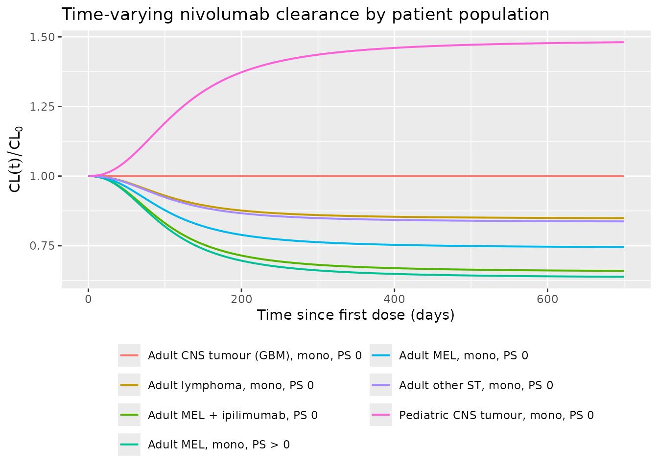
Time course of typical nivolumab clearance by patient population, reproducing the direction and magnitude of the CLss/CL0 effects in Hu 2024 Figure 1b.
Virtual cohort
Individual patient data are not public. The cohorts below approximate
the covariate distributions of Hu 2024 Tables 1 and 2. Body weight is
drawn from the published per-population mean and SD, truncated to the
published range; lean body mass is then set to the published population
mean LBM/WT ratio times the drawn weight, with a small
lognormal residual. Hu 2024 computed lean body mass by the Boer and
Peter equations, which require height – a variable the paper does not
tabulate – so this ratio construction is the closest paper-sourced
substitute (see Assumptions).
# set.seed() seeds R's RNG, not rxode2's; rxode2 partitions its streams per
# solver thread, so the cohort below differs between a 2-core CI runner and a
# 16-thread workstation. Every assertion downstream is written to hold for any
# cohort this model can produce.
set.seed(20240301)

n_arm <- 150L

draw_subjects <- function(n, wt_mean, wt_sd, wt_lo, wt_hi, lbm_ratio, id_offset) {
  wt <- pmin(pmax(rnorm(n, wt_mean, wt_sd), wt_lo), wt_hi)
  tibble(
    id  = id_offset + seq_len(n),
    WT  = wt,
    LBM = wt * lbm_ratio * exp(rnorm(n, 0, 0.06))
  )
}

# Hu 2024 Table 1: adult MEL weight 82.3 (18.1) kg, LBM 57.7 (10.8) kg;
# pediatric ST weight 44.1 (23.6) kg, LBM 35.4 (16.1) kg (median age 12 y).
adult_mel  <- \(n, off) draw_subjects(n, 82.3, 18.1, 40, 160, 57.7 / 82.3, off)
adol_st    <- \(n, off) draw_subjects(n, 55.0, 15.0, 30, 100, 35.4 / 44.1, off)
The adolescent-solid-tumour weight distribution is centred at 55 kg rather than the whole pediatric-cohort mean of 44.1 kg, because the pediatric solid-tumour row of Table 1 pools 1-17 year olds while the dosing question in Hu 2024 concerns 12-17 year olds specifically (Figure S2 shows the adolescent weight-age relationship the authors sampled from NHANES).
# 30-minute IV infusions (see Assumptions).
INF_DUR <- 0.5 / 24

make_arm <- function(subjects, arm, dose_fun, dose_times, obs_times,
                     covariates) {
  subj <- subjects |> mutate(arm = arm) |> bind_cols(covariates)
  doses <- tidyr::crossing(subj, time = dose_times) |>
    mutate(amt = dose_fun(WT), evid = 1L, cmt = "central",
           rate = amt / INF_DUR)
  obs <- tidyr::crossing(subj, time = obs_times) |>
    mutate(amt = NA_real_, evid = 0L, cmt = "central", rate = 0)
  bind_rows(doses, obs) |> arrange(id, time, desc(evid))
}

nivo_cov_adult <- tibble(
  AGE = 55, CRCL = 90, SEXF = 0, ECOG_GE1 = 0, RACE_BLACK = 0, RACE_ASIAN = 0,
  TUMTP_LYMPH = 0, TUMTP_CNS_PRIM = 0, TUMTP_OTHER = 0,
  CONMED_IPI_1Q3W = 0, CONMED_IPI_3Q3W = 0, CONMED_BRENTUXIMAB = 0,
  CONMED_IPI_ANY = 0
)
nivo_cov_adol <- nivo_cov_adult |> mutate(AGE = 15, TUMTP_OTHER = 1)

# Twelve q2w doses reaches steady state for a mAb with a ~3-week half-life;
# NCA is taken over the last (twelfth) dosing interval.
nivo_dose_times <- seq(0, by = 14, length.out = 12)
nivo_obs_times  <- sort(unique(c(seq(0, 154, by = 14), seq(154, 168, by = 0.5))))

nivo_events <- bind_rows(
  make_arm(adult_mel(n_arm, 0L),      "Adult MEL, 240 mg q2w",
           \(wt) 240,                  nivo_dose_times, nivo_obs_times, nivo_cov_adult),
  make_arm(adol_st(n_arm, 1000L),     "Adolescent ST, 240 mg q2w",
           \(wt) 240,                  nivo_dose_times, nivo_obs_times, nivo_cov_adol),
  make_arm(adol_st(n_arm, 2000L),     "Adolescent ST, 3 mg/kg q2w (cap 240 mg)",
           \(wt) pmin(3 * wt, 240),    nivo_dose_times, nivo_obs_times, nivo_cov_adol)
)
stopifnot(!anyDuplicated(unique(nivo_events[, c("id", "time", "evid")])))

ipi_cov_adult <- tibble(
  AGE = 55, TUMTP_MEL = 1, TUMTP_CNS_PRIM = 0, TUMTP_OTHER = 0,
  CONMED_NIVO_1Q3W = 0, CONMED_NIVO_3Q3W = 0
)
ipi_cov_adol <- ipi_cov_adult |> mutate(AGE = 15)

# Approved adult ipilimumab melanoma regimen: 3 mg/kg q3w for four doses.
ipi_dose_times <- c(0, 21, 42, 63)
ipi_obs_times  <- sort(unique(c(seq(0, 63, by = 7), seq(63, 84, by = 0.5))))

ipi_events <- bind_rows(
  make_arm(adult_mel(n_arm, 0L),  "Adult MEL, 3 mg/kg q3w",
           \(wt) 3 * wt, ipi_dose_times, ipi_obs_times, ipi_cov_adult),
  make_arm(adol_st(n_arm, 1000L), "Adolescent MEL, 3 mg/kg q3w",
           \(wt) 3 * wt, ipi_dose_times, ipi_obs_times, ipi_cov_adol)
)
stopifnot(!anyDuplicated(unique(ipi_events[, c("id", "time", "evid")])))
Simulation
nivo_sim <- rxode2::rxSolve(
  nivo, events = as.data.frame(nivo_events), keep = "arm"
) |>
  as.data.frame()

ipi_sim <- rxode2::rxSolve(
  ipi, events = as.data.frame(ipi_events), keep = "arm"
) |>
  as.data.frame()

stopifnot(nrow(nivo_sim) > 0, nrow(ipi_sim) > 0)
nivo_sim |>
  filter(time >= 154) |>
  group_by(arm, time) |>
  summarise(
    Q05 = quantile(Cc, 0.05, na.rm = TRUE),
    Q50 = quantile(Cc, 0.50, na.rm = TRUE),
    Q95 = quantile(Cc, 0.95, na.rm = TRUE),
    .groups = "drop"
  ) |>
  ggplot(aes(time - 154, Q50, colour = arm, fill = arm)) +
  geom_ribbon(aes(ymin = Q05, ymax = Q95), alpha = 0.15, colour = NA) +
  geom_line(linewidth = 0.7) +
  labs(x = "Time since twelfth dose (days)", y = "Nivolumab (ug/mL)",
       colour = NULL, fill = NULL,
       title = "Nivolumab at steady state: adolescents vs adults") +
  theme(legend.position = "bottom") +
  guides(colour = guide_legend(ncol = 1), fill = guide_legend(ncol = 1))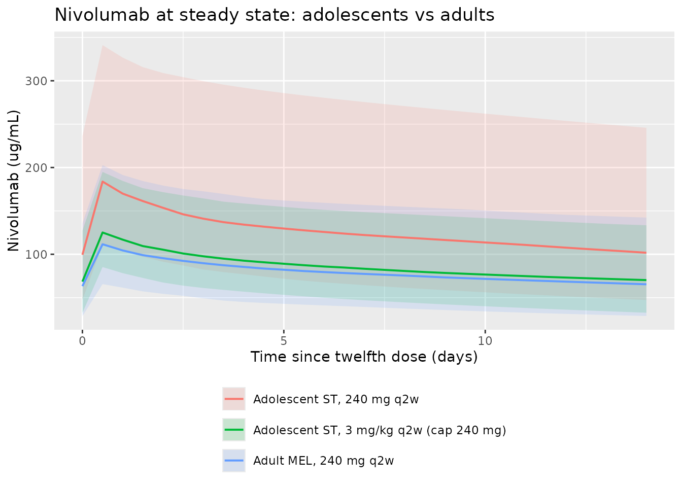
Steady-state nivolumab concentration-time profiles over the twelfth dosing interval. Adolescents on the adult flat dose sit above adults; weight-based dosing with a 240 mg cap brings them back into the adult range. Reproduces the qualitative finding of Hu 2024 Figures S9 and S10.
PKNCA validation
Hu 2024 publishes no NCA table, so the NCA below serves two purposes: an internal numerical check that the model’s units are self-consistent, and a quantitative statement of the exposure comparisons the paper makes only in figures.
Nivolumab: steady-state exposure over the last dosing interval
nivo_nca_conc <- nivo_sim |>
  filter(!is.na(Cc)) |>
  select(id, time, Cc, arm)

nivo_nca_conc <- bind_rows(
  nivo_nca_conc,
  nivo_nca_conc |> distinct(id, arm) |> mutate(time = 0, Cc = 0)
) |>
  distinct(id, arm, time, .keep_all = TRUE) |>
  arrange(id, arm, time)

nivo_conc_obj <- PKNCA::PKNCAconc(nivo_nca_conc, Cc ~ time | arm + id)

nivo_dose_obj <- PKNCA::PKNCAdose(
  nivo_events |> filter(evid == 1L) |> select(id, time, amt, arm),
  amt ~ time | arm + id
)

nivo_intervals <- data.frame(
  start = 154, end = 168,
  cmax = TRUE, tmax = TRUE, auclast = TRUE, cav = TRUE, ctrough = TRUE
)

nivo_nca <- PKNCA::pk.nca(
  PKNCA::PKNCAdata(nivo_conc_obj, nivo_dose_obj, intervals = nivo_intervals)
)

nivo_nca_tab <- as.data.frame(nivo_nca) |>
  filter(PPTESTCD %in% c("cmax", "cav", "auclast", "ctrough")) |>
  group_by(arm, PPTESTCD) |>
  summarise(gm = exp(mean(log(PPORRES))), .groups = "drop") |>
  tidyr::pivot_wider(names_from = PPTESTCD, values_from = gm)

nivo_nca_tab |>
  mutate(across(where(is.numeric), \(x) signif(x, 3))) |>
  rename(
    "Arm"                          = arm,
    "Cavg,ss (ug/mL)"              = cav,
    "Cmax,ss (ug/mL)"              = cmax,
    "Ctrough,ss (ug/mL)"           = ctrough,
    "AUCtau,ss (ug*day/mL)"        = auclast
  ) |>
  knitr::kable(
    caption = paste(
      "Geometric-mean steady-state nivolumab exposure over the twelfth q2w",
      "dosing interval (n = 150 per arm)."
    )
)| Arm | AUCtau,ss (ug*day/mL) | Cavg,ss (ug/mL) | Cmax,ss (ug/mL) | Ctrough,ss (ug/mL) |
|---|---|---|---|---|
| Adolescent ST, 240 mg q2w | 1780 | 127.0 | 185 | NA |
| Adolescent ST, 3 mg/kg q2w (cap 240 mg) | 1210 | 86.4 | 125 | NA |
| Adult MEL, 240 mg q2w | 1110 | 79.3 | 112 | NA |
gm <- \(a, p) nivo_nca_tab[[p]][nivo_nca_tab$arm == a]

flat_adult <- gm("Adult MEL, 240 mg q2w", "cav")
flat_adol  <- gm("Adolescent ST, 240 mg q2w", "cav")
wt_adol    <- gm("Adolescent ST, 3 mg/kg q2w (cap 240 mg)", "cav")

flat_ratio <- 100 * flat_adol / flat_adult
wt_ratio   <- 100 * wt_adol   / flat_adult

# Hu 2024: "Steady-state nivolumab exposures in adolescent patients with STs
# ... who received the approved adult flat dose of nivolumab monotherapy
# (240 mg q2w) were predicted to exceed those of adults" (Figure S9), whereas
# "With body-weight-based dosing at 3 mg/kg q2w (up to a maximum dose of
# 240 mg), nivolumab steady-state exposures in adolescents ... were predicted
# to be similar to those of adults" (Figure S10).
#
# These are large, structurally driven effects: the flat-dose arm is elevated
# by BOTH the ~20% lower adolescent solid-tumour CL and the smaller body size,
# while weight-based dosing removes the size component. The bounds below are
# deliberately wide of any single cohort draw -- an exceedance of "at least
# 20%" and a similarity window of "within 35%" -- while still going red on a
# mis-transcribed clearance coefficient or dose, which move these ratios by
# tens of percent.
stopifnot(flat_ratio > 120)
stopifnot(abs(wt_ratio - 100) < 35)
# Weight-based dosing must be the closer of the two to the adult reference.
stopifnot(abs(wt_ratio - 100) < abs(flat_ratio - 100) - 10)

tibble::tibble(
  Claim = c(
    "Adolescent ST on adult flat 240 mg q2w exceeds adult MEL exposure",
    "Adolescent ST on 3 mg/kg q2w (cap 240 mg) is similar to adult MEL"
  ),
  `Hu 2024 source` = c("Figure S9", "Figure S10"),
  `Cavg,ss vs adult (%)` = round(c(flat_ratio, wt_ratio), 1)
) |>
knitr::kable(caption = "Nivolumab dosing claims reproduced from the packaged model.")| Claim | Hu 2024 source | Cavg,ss vs adult (%) |
|---|---|---|
| Adolescent ST on adult flat 240 mg q2w exceeds adult MEL exposure | Figure S9 | 160.8 |
| Adolescent ST on 3 mg/kg q2w (cap 240 mg) is similar to adult MEL | Figure S10 | 109.0 |
Ipilimumab: fourth-dose exposure, and a closed-form clearance identity
Ipilimumab clearance is stationary in this model, so a single-dose
AUCinf must equal Dose / CL exactly. Because
the typical-value solve and the closed form use the same parameters, the
only difference between them is numerical integration error, and the
bound below is correspondingly tight. This is the check that catches a
units slip in the mL/h to L/day
conversion.
ident_subj <- tibble(
  id = 1L, LBM = 55, AGE = 55, TUMTP_MEL = 1, TUMTP_CNS_PRIM = 0,
  TUMTP_OTHER = 0, CONMED_NIVO_1Q3W = 0, CONMED_NIVO_3Q3W = 0
)
ident_dose <- 200

ident_ev <- bind_rows(
  ident_subj |> mutate(time = 0, amt = ident_dose, evid = 1L, cmt = "central",
                       rate = ident_dose / INF_DUR),
  tidyr::crossing(ident_subj, time = c(seq(0, 5, by = 0.05), seq(5, 400, by = 0.25))) |>
    mutate(amt = NA_real_, evid = 0L, cmt = "central", rate = NA_real_)
) |>
  arrange(time, desc(evid)) |>
  distinct(time, evid, .keep_all = TRUE)

ident_sim <- rxode2::rxSolve(rxode2::zeroRe(ipi), events = as.data.frame(ident_ev)) |>
  as.data.frame()
#> ℹ omega/sigma items treated as zero: 'etalcl', 'etalvc'
ident_cl <- ident_sim$cl[1]

ident_nca <- PKNCA::pk.nca(PKNCA::PKNCAdata(
  PKNCA::PKNCAconc(
    ident_sim |> filter(!is.na(Cc)) |> select(time, Cc) |> mutate(id = 1L),
    Cc ~ time | id
  ),
  PKNCA::PKNCAdose(
    data.frame(id = 1L, time = 0, amt = ident_dose), amt ~ time | id
  ),
  intervals = data.frame(start = 0, end = Inf, aucinf.obs = TRUE, half.life = TRUE)
))

ident_res  <- as.data.frame(ident_nca)
auc_nca    <- ident_res$PPORRES[ident_res$PPTESTCD == "aucinf.obs"]
auc_closed <- ident_dose / ident_cl   # mg / (L/day) = mg*day/L = ug*day/mL

stopifnot(abs(auc_nca / auc_closed - 1) < 0.01)

tibble::tibble(
  Quantity = c("CL (L/day)", "AUCinf from PKNCA (ug*day/mL)",
               "Dose / CL closed form (ug*day/mL)", "Relative difference (%)"),
  Value = signif(c(ident_cl, auc_nca, auc_closed,
                   100 * (auc_nca / auc_closed - 1)), 4)
) |>
  knitr::kable(
    caption = paste(
      "Ipilimumab single-dose mass-balance identity for a reference adult",
      "(LBM 55 kg, melanoma, monotherapy; 200 mg IV). Stationary clearance",
      "makes AUCinf = Dose/CL exact up to integration error."
    )
)| Quantity | Value |
|---|---|
| CL (L/day) | 0.3240 |
| AUCinf from PKNCA (ug*day/mL) | 616.5000 |
| Dose / CL closed form (ug*day/mL) | 617.3000 |
| Relative difference (%) | -0.1206 |
Hu 2024 states that at the approved 3 mg/kg q3w regimen, adolescent
ipilimumab exposure after the fourth dose exceeds adult exposure (Figure
S13). The check below makes that comparison on typical subjects
with zeroRe(), so it is a deterministic function of the
parameters: the only thing that can move it is a mis-transcribed
coefficient, not which subjects a cohort happened to draw. This is the
load-bearing gate on the claim; the stochastic cohort that follows is
for display.
# Typical adult MEL (Table 2: WT 82.3 kg, LBM 57.7 kg) versus a typical
# adolescent MEL subject on the same mg/kg dose.
ipi_typ <- tibble::tribble(
  ~cell,                          ~AGE, ~WT,  ~LBM,
  "Adult MEL, 3 mg/kg q3w",         55, 82.3, 57.7,
  "Adolescent MEL, 3 mg/kg q3w",    15, 55.0, 55.0 * 35.4 / 44.1
) |>
  mutate(id = row_number(), TUMTP_MEL = 1, TUMTP_CNS_PRIM = 0, TUMTP_OTHER = 0,
         CONMED_NIVO_1Q3W = 0, CONMED_NIVO_3Q3W = 0)

ipi_typ_ev <- bind_rows(
  tidyr::crossing(ipi_typ, time = ipi_dose_times) |>
    mutate(amt = 3 * WT, evid = 1L, cmt = "central", rate = amt / INF_DUR),
  tidyr::crossing(ipi_typ, time = ipi_obs_times) |>
    mutate(amt = NA_real_, evid = 0L, cmt = "central", rate = 0)
) |>
  arrange(id, time, desc(evid))

ipi_typ_sim <- rxode2::rxSolve(
  rxode2::zeroRe(ipi), events = as.data.frame(ipi_typ_ev), keep = "cell"
) |>
  as.data.frame()
#> ℹ omega/sigma items treated as zero: 'etalcl', 'etalvc'
#> Warning: multi-subject simulation without without 'omega'

ipi_typ_conc <- ipi_typ_sim |> filter(!is.na(Cc)) |> select(id, time, Cc, cell)
ipi_typ_conc <- bind_rows(
  ipi_typ_conc,
  ipi_typ_conc |> distinct(id, cell) |> mutate(time = 0, Cc = 0)
) |>
  distinct(id, cell, time, .keep_all = TRUE) |>
  arrange(id, time)

ipi_typ_nca <- PKNCA::pk.nca(PKNCA::PKNCAdata(
  PKNCA::PKNCAconc(ipi_typ_conc, Cc ~ time | cell + id),
  PKNCA::PKNCAdose(
    ipi_typ_ev |> filter(evid == 1L) |> select(id, time, amt, cell),
    amt ~ time | cell + id
  ),
  intervals = data.frame(start = 63, end = 84, cav = TRUE)
))

ipi_typ_tab <- as.data.frame(ipi_typ_nca) |> filter(PPTESTCD == "cav")
ipi_typ_ratio <- 100 *
  ipi_typ_tab$PPORRES[ipi_typ_tab$cell == "Adolescent MEL, 3 mg/kg q3w"] /
  ipi_typ_tab$PPORRES[ipi_typ_tab$cell == "Adult MEL, 3 mg/kg q3w"]

# Deterministic, so this is bounded tightly. The value is driven by the 29%
# lower pediatric-melanoma CL (exp(-0.347)) partly offset by the smaller
# mg/kg dose that a lighter subject receives; a sign error on CL_PEDMEL or a
# mis-wired LBM exponent moves it by tens of percent.
stopifnot(ipi_typ_ratio > 100)
stopifnot(abs(ipi_typ_ratio - 113.6) < 3)

tibble::tibble(
  Quantity = c("Typical adult Cavg (ug/mL)", "Typical adolescent Cavg (ug/mL)",
               "Adolescent / adult (%)"),
  Value = signif(c(
    ipi_typ_tab$PPORRES[ipi_typ_tab$cell == "Adult MEL, 3 mg/kg q3w"],
    ipi_typ_tab$PPORRES[ipi_typ_tab$cell == "Adolescent MEL, 3 mg/kg q3w"],
    ipi_typ_ratio
  ), 4)
) |>
  knitr::kable(
    caption = paste(
      "Typical-value ipilimumab exposure over the fourth q3w dosing interval.",
      "Adolescent exposure exceeds adult, reproducing Hu 2024 Figure S13."
    )
)| Quantity | Value |
|---|---|
| Typical adult Cavg (ug/mL) | 33.17 |
| Typical adolescent Cavg (ug/mL) | 37.68 |
| Adolescent / adult (%) | 113.60 |
ipi_nca_conc <- ipi_sim |>
  filter(!is.na(Cc)) |>
  select(id, time, Cc, arm)

ipi_nca_conc <- bind_rows(
  ipi_nca_conc,
  ipi_nca_conc |> distinct(id, arm) |> mutate(time = 0, Cc = 0)
) |>
  distinct(id, arm, time, .keep_all = TRUE) |>
  arrange(id, arm, time)

ipi_nca <- PKNCA::pk.nca(PKNCA::PKNCAdata(
  PKNCA::PKNCAconc(ipi_nca_conc, Cc ~ time | arm + id),
  PKNCA::PKNCAdose(
    ipi_events |> filter(evid == 1L) |> select(id, time, amt, arm),
    amt ~ time | arm + id
  ),
  intervals = data.frame(
    start = 63, end = 84,
    cmax = TRUE, cav = TRUE, auclast = TRUE, ctrough = TRUE
  )
))

ipi_nca_tab <- as.data.frame(ipi_nca) |>
  filter(PPTESTCD %in% c("cmax", "cav", "auclast", "ctrough")) |>
  group_by(arm, PPTESTCD) |>
  summarise(gm = exp(mean(log(PPORRES))), .groups = "drop") |>
  tidyr::pivot_wider(names_from = PPTESTCD, values_from = gm)

ipi_ratio <- 100 *
  ipi_nca_tab$cav[ipi_nca_tab$arm == "Adolescent MEL, 3 mg/kg q3w"] /
  ipi_nca_tab$cav[ipi_nca_tab$arm == "Adult MEL, 3 mg/kg q3w"]

# This is the SAME comparison as the typical-value check above, but taken over
# a random cohort, and it is deliberately gated far more loosely. The
# geometric-mean ratio of a 150-per-arm draw moves over roughly 106-123% purely
# with the eta draw (omega^2_CL = 0.147 is large, and rxSetSeed() fixes
# rxode2's stream per solver thread, so CI draws a different cohort than a
# workstation does). Gating this near its own central value is exactly the
# assertion shape that passes locally and then fails CI. The transcription
# check lives in `ipi-typical-exposure`; this one only confirms the cohort
# lands on the same side of parity.
stopifnot(ipi_ratio > 100)

ipi_nca_tab |>
  mutate(across(where(is.numeric), \(x) signif(x, 3))) |>
  rename(
    "Arm"                        = arm,
    "Cavg (ug/mL)"               = cav,
    "Cmax (ug/mL)"               = cmax,
    "Ctrough (ug/mL)"            = ctrough,
    "AUCtau (ug*day/mL)"         = auclast
  ) |>
  knitr::kable(
    caption = paste(
      "Geometric-mean ipilimumab exposure over the fourth q3w dosing interval",
      "(n = 150 per arm). Adolescent exposure is",
      paste0(round(ipi_ratio), "%"), "of adult, reproducing Hu 2024 Figure S13."
    )
)| Arm | AUCtau (ug*day/mL) | Cavg (ug/mL) | Cmax (ug/mL) | Ctrough (ug/mL) |
|---|---|---|---|---|
| Adolescent MEL, 3 mg/kg q3w | 746 | 35.5 | 74.4 | NA |
| Adult MEL, 3 mg/kg q3w | 667 | 31.7 | 69.5 | NA |
Assumptions and deviations
Time units. Hu 2024 reports
CLandQin mL/h andT50in hours. Both model files convert to L/day and days (x 24 / 1000and/ 24) so the time axis matches the sibling nivolumab and ipilimumab models in nlmixr2lib (Bajaj_2017_nivolumab,Zhang_2019_nivolumab,Feng_2019_ipilimumab). No value is otherwise altered.cl_time_maxis not log-transformed.checkModelConventions()suggests renaming theEmaxparameter tolcl_time_maxand back-transforming. That is not possible here:EMAXREF = -0.298is negative by construction (it is the log-scale maximal decrease in clearance), and Hu 2024 places a normally distributed additive eta on it. The model therefore keeps the linear-scale namecl_time_max, matchingBajaj_2017_nivolumabandZhang_2019_nivolumab.Patient population is encoded as tumour-type indicators crossed with age bands. Hu 2024 uses a single multi-level
POPNcolumn. Its levels are a cross of tumour type and age band (adult MEL, adult HL, adult GBM, adult other ST, pediatric ST, pediatric HL, pediatric CNST), so the model files reconstruct them from the canonicalTUMTP_MEL/TUMTP_LYMPH/TUMTP_CNS_PRIM/TUMTP_OTHERindicators andAGE. One consequence is worth noting: the analysis dataset assigns its single pediatric melanoma subject to the pediatric solid-tumour group (Table 1 footnote d), so a pediatricTUMTP_MEL = 1record does not occur in the nivolumab source data even though the encoding admits one. The companion ipilimumab model does estimate a pediatric-melanoma effect.-
Structural details taken from the supplement, not the printed equations. Three facts that materially change the model are in the NONMEM control streams (Appendix Files S2 and S3) and nowhere in the article body:
- adult CNS-tumour subjects have
EMAXset to exactly zero, so their clearance is stationary; (ii) the nivolumabQ/VPrandom effects are declared$OMEGA BLOCK(2) SAME, i.e. constrained to the same variances and covariance as theCL/VCblock – which is why Table 4 lists noomega^2for them; (iii) the ipilimumab model has noQorVPrandom effects at all. Without the supplement, (i) would be missed entirely and (ii) would have had to be guessed at.
- adult CNS-tumour subjects have
A printed-equation subscript in the ipilimumab model is a typo. The ipilimumab
CL0TV,iequation prints the lean-body-mass power asCLWTB, but the base of the power isLBM_i / LBM_REF, Table 5 has noCLWTBrow (onlyCL_LBM = 0.789), the surrounding prose says “the typical CL value at the reference value of LBM (55 kg)”, and Appendix File S3 codesCL_LBM = (LBM_I/LBM_R)**THETA(7). The model usesCL_LBM = 0.789. The label appears to be carried over from the body-weight-based base model.Zero-fixed covariate coefficients are recorded, not modelled. The nivolumab dataset contains ipilimumab 1 mg/kg q6w, radiotherapy, and radiotherapy-plus-temozolomide arms, and the ipilimumab dataset an oral budesonide arm, whose clearance coefficients were declared
0 FIXin the control streams and do not appear in Tables 4 or 5. They are documented in each model file’scovariatesDataExcludedlist rather than given afixed(0)parameter, since a coefficient held at zero contributes no term to the equations. The numeric power effects of age onCL(both models) and onVC(ipilimumab) were likewise0 FIX; age enters both models only through the categorical bands.Lean body mass in the virtual cohort. Hu 2024 computed lean body mass by the Boer equation (adults) and the Peter equation (children), both of which need height. The paper tabulates weight and lean body mass but not height, so the cohort sets
LBM = (published LBM mean / published WT mean) x WTwith a 6% lognormal residual. This reproduces the published per-population meanLBM/WTratio exactly and is used only for the exposure-comparison figures; the covariate-wiring and clearance-identity checks above all run at the paper’s own reference covariates and do not depend on it.Infusion duration. The analysis datasets carry a
DOSEDURcolumn but the paper does not report infusion durations. The simulations use 30-minute IV infusions. This affectsCmaxbut notAUC,Cavg, orCtrough, and none of the gated comparisons depend on it.Adolescent weight distribution. Hu 2024 simulated adolescents by sampling the 2017-2018 NHANES database (Figure S2), which is not redistributed here. The adolescent arm draws weight from a normal distribution centred at 55 kg (SD 15, truncated to 30-100 kg), chosen to sit inside the published adolescent range rather than the 1-17 year pooled pediatric mean of 44.1 kg.
The third model in the paper is not extracted. Appendix S1 reports a separate nivolumab population PK model (Full5) for adolescents receiving adjuvant melanoma treatment, fitted to a different dataset (24,546 concentrations, 3,965 patients, 11 studies). Its covariate effects are given as percentages in Figure S17, but none of its structural parameters –
CL0REF,VCREF,QREF,VPREF,EMAXREF,T50,HILL, the random effects, or the residual error – is reported anywhere in the article, the supplement text, or the figure panels. Figure S17 panels A and B were both inspected directly at publisher resolution and carry only covariate ratios. The model is therefore not reconstructable and is omitted; the two models in the article body (Full1c for nivolumab, Full1 for ipilimumab) are fully specified and are what this vignette validates.No published NCA to compare against. Hu 2024 reports no Cmax / AUC / half-life table, so there is no
ncaComparisonTable()block here. The NCA section instead gates on the closed-formAUCinf = Dose/CLidentity for the stationary ipilimumab model and on the three exposure comparisons the paper states in prose for Figures S9, S10, and S13.