Model and source
- Citation: Okada A, Sera S, Nagai N. Appropriate use of triazolam in elderly patients considering a quantitative benefit-risk assessment based on the pharmacokinetic-pharmacodynamic modeling and simulation approach supported by real-world data. BMC Pharmacol Toxicol. 2024;25:60. doi:10.1186/s40360-024-00777-z
- Description: One-compartment first-order-absorption population PK model for oral triazolam in young and elderly adults (Okada 2024, Table 3), coupled to an effect-compartment linear direct-effect PK/PD layer for two parallel endpoints: sedation (visual analogue scale, mm) and cognitive function (percent change). Age enters apparent volume and apparent clearance as a power law centred at 30 years (Eq 1), and a continuous CYP3A drug-interaction AUC ratio (AUCR) divides apparent clearance, so the model reproduces the paper’s benefit-risk simulations of triazolam dose in the elderly with and without CYP3A inhibitors. The model was fit to digitised mean young-adult and elderly concentration/effect profiles from Greenblatt 1991 (N Engl J Med 324:1691-8); no inter-individual variability was estimated.
- Article: BMC Pharmacol Toxicol. 2024;25:60 (PMC11370030, open access)
Okada, Sera and Nagai combined a Japanese pharmacovigilance analysis (JADER, FAERS and the National Database of Health Insurance Claims) with a pharmacokinetic/pharmacodynamic model in order to recommend a triazolam dose for elderly patients. Only the PK/PD half of the paper is represented here; the disproportionality analysis (Table 2) informed the clinical framing but is not a model.
The model has three layers:
-
PK – one compartment with first-order oral
absorption. Age enters both the apparent volume and the apparent
clearance as a power law centred at 30 years (Eq 1). A continuous
drug-interaction AUC ratio,
AUCR, divides apparent clearance. -
Link – a single effect compartment equilibrating
with plasma at rate
Keo. The authors adopted it because an anticlockwise hysteresis loop was observed between plasma concentration and effect; the effect-compartment model gave OFV 193.7 against 223.5 (direct-response linear) and 225.2 (direct-response Emax). - PD – two parallel linear direct effects on the effect-site concentration: sedation (visual analogue scale, mm) and cognitive function (percent). Both are change-from-baseline measures and carry no intercept.
The paper’s clinical conclusions are read off three simulations, which this vignette reproduces as quantitative gates:
- Simulation I – time for plasma triazolam to fall below the 0.44 ng/mL adverse-event threshold after 0.25 mg in a healthy young adult.
- Simulation II – the elderly dose that reaches the threshold at that same time.
-
Simulation III – with 0.0625 mg in an elderly
patient, the largest
AUCRfor which the threshold is still reached by that time.
Population
Okada 2024 enrolled no new subjects. Mean plasma triazolam
concentration, sedation and cognitive-function time courses were
digitised with WebPlotDigitizer 4.3 from Greenblatt DJ, Harmatz JS,
Shapiro L, Engelhardt N, Gouthro TA, Shader RI, Sensitivity to
triazolam in the elderly, N Engl J Med 1991;324(24):1691-8 (the
paper’s reference 18). That source supplied only group mean profiles,
for a young cohort (30 years, 72 kg) and an elderly cohort (69 years, 69
kg), after a single 0.25 mg oral dose. Okada 2024 does not restate the
per-cohort subject counts, so n_subjects is deliberately
left unset in the model metadata rather than inferred.
Because only two group means were fitted, inter-individual
variability was deliberately not estimated (Methods,
“Pharmacokinetic-pharmacodynamic modeling”), and the packaged model
correspondingly carries no eta terms. Only two ages
informed the age power law, so the paper’s own Limitations section
states that “indications for ages other than 30 or 69 years … are
unknown”. Estimation used Certara NLME 8.1.
The AUCR values used to drive the interaction
simulations were not measured in this cohort. They were extracted from
the University of Washington Drug Interaction Database as the 15
co-medications whose triazolam AUC ratio is at least 1.25 (Table 1).
The same information is available programmatically via the model’s
population metadata
(readModelDb("Okada_2024_triazolam")()$population).
Source trace
The per-parameter origin is recorded as an in-file comment next to
each ini() entry in
inst/modeldb/specificDrugs/Okada_2024_triazolam.R. The
table below collects them in one place for review. Every value comes
from Table 3 or its footnote; the paper reports no supplementary
parameter table.
| Equation / parameter | Value | Source location |
|---|---|---|
lka (Ka) |
3.16 1/h (CV 5.27%) | Table 3, Ka = theta1
|
lvc (Vd/F at age 30) |
119 L (CV 1.86%) | Table 3, theta2
|
e_age_vc |
-0.49 (CV 6.53%) | Table 3, theta4
|
lcl (CL/F at age 30) |
0.47 L/h/kg (CV 1.92%) | Table 3, theta3
|
e_age_cl |
-0.53 (CV 4.30%) | Table 3, theta5
|
propSd |
0.0620 (6.20%, CV 10.8%) | Table 3, sigma (%); Eq 2 |
lke0 (Keo) |
3.42 1/h (CV 12.6%) | Table 3, Keo
|
slope_sedation |
12.1 mm per ng/mL (CV 1.05%) | Table 3 footnote, “Sedation = 12.1 x concentration” |
slope_cognitive |
-11.0 % per ng/mL (CV 3.14%) | Table 3 footnote, “Cognitive function = -11.0 x concentration” |
addSd_sedation |
6.81 mm (CV 21.8%) | Table 3, sigma Sedation (mm); Eq 3 |
addSd_cognitive |
3.27 % (CV 14.5%) | Table 3, sigma Cognitive function (%); Eq 3 |
Age power law theta * (age/30)^theta_cov
|
n/a | Eq 1 (Methods, “Pharmacokinetic-pharmacodynamic modeling”) |
Vd = theta2 * (age/30)^theta4 |
n/a | Table 3, parameter-name column |
CL = theta3 * (age/30)^theta5 * 1/AUCR |
n/a | Table 3, parameter-name column; Methods, “when the dose is constant, the inverse of AUCR was added as a covariate of clearance” |
CL/F multiplied by body weight |
n/a | Table 3 unit of theta3 (L/hr/kg) |
| One compartment, first-order absorption | n/a | Methods; Results, “a one-compartment model including a first-order absorption process best representing the changes in blood concentration” |
Effect compartment
d/dt(effect) = Keo * (Cc - effect)
|
n/a | Results, “an anticlockwise hysteresis loop … therefore, an effect compartment model was adopted” |
| Linear (not Emax) PD, no intercept | n/a | Results, “drug susceptibility against concentration in the effect compartment exhibited a positive linear correlation”; Table 3 footnote gives slope-only relations |
| Proportional residual error on PK | n/a | Methods Eq 2 |
| Additive residual error on both PD endpoints | n/a | Methods Eq 3 |
| Adverse-event threshold 0.44 ng/mL (sedation) | n/a | Results (ROC; sensitivity 0.85, specificity 0.90) |
| Cognitive-function threshold 0.58 ng/mL | n/a | Results (ROC; sensitivity 1.00, specificity 1.00) |
AUCR values for 15 co-medications |
1.31-40.7 | Table 1 |
The unit conversion Cc = central / vc * 1000 (mg/L to
ng/mL) is a derived scaling, not a published value; it follows from
units$dosing = "mg",
units$concentration = "ng/mL" and volumes in litres.
Virtual cohort
The published figures are typical-value predictions, not visual predictive checks: the model has no inter-individual variability, so a single deterministic subject per arm reproduces each published curve exactly. Two cohort sets are built.
-
Figure 1 set – five arms: 30 years / 72 kg at 0.25
and 0.125 mg, and 69 years / 69 kg at 0.25, 0.125 and 0.0625 mg, all
with
AUCR = 1. -
Figure 2 set – five arms: 69 years / 69 kg at
0.0625 mg with
AUCR= 1, 2.27 (the paper’s acceptable ceiling), 3.38 (diltiazem), 5.26 (clarithromycin) and 27.1 (itraconazole).
Every endpoint in this model is an algebraic observable
(Cc, sedation and cognitive are
all expressions, not ODE states), so observation rows carry
dvid = 1 with a blank cmt rather than naming a
compartment. All three observable columns are returned on every solved
row.
# One deterministic subject per arm; far below the 200-per-arm cap.
make_arm <- function(id, label, dose, age, wt, aucr, tmax = 24, n_obs = 241) {
  dosing <- data.frame(
    id = id, time = 0, amt = dose, evid = 1L,
    cmt = "depot", dvid = NA_integer_
  )
  obs <- data.frame(
    id = id, time = seq(0, tmax, length.out = n_obs), amt = NA_real_, evid = 0L,
    cmt = NA_character_, dvid = 1L
  )
  out <- rbind(dosing, obs)
  out$arm <- label
  out$AGE <- age
  out$WT <- wt
  out$AUCR <- aucr
  out[order(out$time, out$evid == 0L), ]
}

fig1_arms <- tibble::tribble(
  ~label,                  ~dose,   ~age, ~wt,
  "30 y, 0.25 mg",         0.25,    30,   72,
  "30 y, 0.125 mg",        0.125,   30,   72,
  "69 y, 0.25 mg",         0.25,    69,   69,
  "69 y, 0.125 mg",        0.125,   69,   69,
  "69 y, 0.0625 mg",       0.0625,  69,   69
)

events_fig1 <- dplyr::bind_rows(lapply(seq_len(nrow(fig1_arms)), function(i) {
  make_arm(
    id = i, label = fig1_arms$label[i], dose = fig1_arms$dose[i],
    age = fig1_arms$age[i], wt = fig1_arms$wt[i], aucr = 1
  )
}))

fig2_arms <- tibble::tribble(
  ~label,                          ~aucr,
  "AUCR 1 (no inhibitor)",          1.00,
  "AUCR 2.27 (paper ceiling)",      2.27,
  "AUCR 3.38 (diltiazem)",          3.38,
  "AUCR 5.26 (clarithromycin)",     5.26,
  "AUCR 27.1 (itraconazole)",      27.10
)

events_fig2 <- dplyr::bind_rows(lapply(seq_len(nrow(fig2_arms)), function(i) {
  make_arm(
    id = 100L + i, label = fig2_arms$label[i], dose = 0.0625,
    age = 69, wt = 69, aucr = fig2_arms$aucr[i]
  )
}))

# IDs must be disjoint across arms or rxSolve silently merges subjects.
stopifnot(!anyDuplicated(unique(events_fig1[, c("id", "time", "evid")])))
stopifnot(!anyDuplicated(unique(events_fig2[, c("id", "time", "evid")])))
stopifnot(length(intersect(events_fig1$id, events_fig2$id)) == 0L)
Simulation
mod <- readModelDb("Okada_2024_triazolam")

sim_fig1 <- rxode2::rxSolve(mod, events = events_fig1, keep = c("arm", "AGE", "AUCR")) |>
  as.data.frame()
#> Warning: multi-subject simulation without without 'omega'
sim_fig2 <- rxode2::rxSolve(mod, events = events_fig2, keep = c("arm", "AGE", "AUCR")) |>
  as.data.frame()
#> Warning: multi-subject simulation without without 'omega'

# Sanity: the model carries no IIV, so Cc is the typical-value prediction.
stopifnot(all(c("Cc", "sedation", "cognitive") %in% names(sim_fig1)))
Replicate published figures
threshold <- 0.44 # ng/mL, ROC-derived sedation threshold (Results)
t_young <- 5.95   # h, Simulation I result reported by the paper

sim_fig1 |>
  mutate(arm = factor(arm, levels = fig1_arms$label)) |>
  ggplot(aes(time, Cc, colour = arm, linetype = AGE == 30)) +
  geom_line(linewidth = 0.7) +
  geom_hline(yintercept = threshold, linetype = "dotted") +
  geom_vline(xintercept = t_young, linetype = "dotted") +
  scale_linetype_manual(values = c("TRUE" = "22", "FALSE" = "solid"), guide = "none") +
  coord_cartesian(xlim = c(0, 12), ylim = c(0, 3)) +
  labs(
    x = "Time (h)", y = "Plasma triazolam (ng/mL)", colour = NULL,
    title = "Figure 1 - simulated plasma triazolam in young and elderly adults",
    caption = paste(
      "Dashed lines: 30 years. Solid lines: 69 years. Dotted horizontal line:",
      "0.44 ng/mL cut-off; dotted vertical line: 5.95 h.",
      "Replicates Figure 1 of Okada 2024."
    )
  )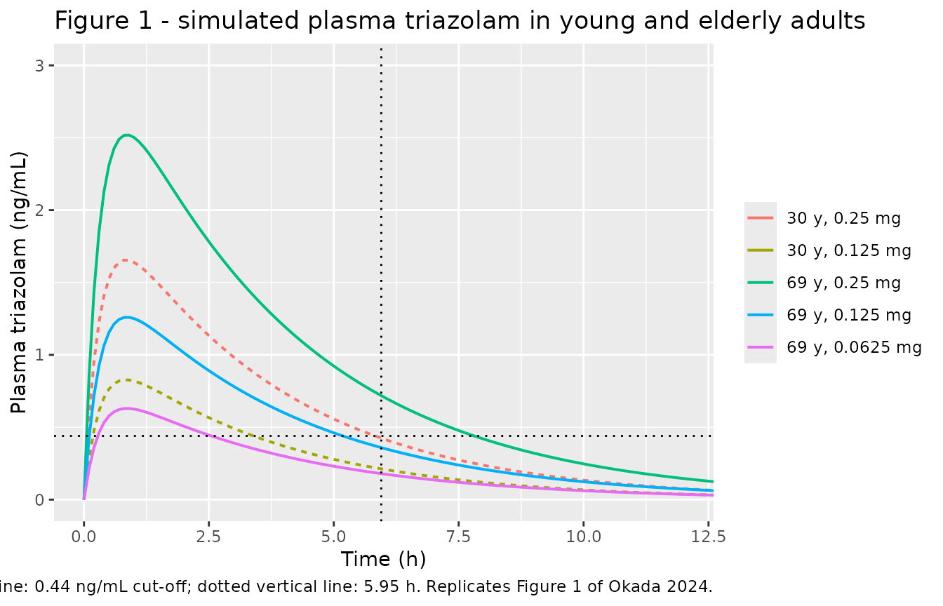
Replicates Figure 1 of Okada 2024.
sim_fig2 |>
  mutate(arm = factor(arm, levels = fig2_arms$label)) |>
  select(time, arm, Cc, sedation, cognitive) |>
  pivot_longer(c(Cc, sedation, cognitive), names_to = "endpoint", values_to = "value") |>
  mutate(endpoint = factor(
    endpoint,
    levels = c("Cc", "sedation", "cognitive"),
    labels = c("Plasma triazolam (ng/mL)", "Sedation (VAS, mm)",
               "Cognitive function (%)")
  )) |>
  ggplot(aes(time, value, colour = arm)) +
  geom_line(linewidth = 0.7) +
  geom_hline(
    data = data.frame(
      endpoint = factor("Plasma triazolam (ng/mL)",
                        levels = c("Plasma triazolam (ng/mL)", "Sedation (VAS, mm)",
                                   "Cognitive function (%)")),
      y = threshold
    ),
    aes(yintercept = y), linetype = "dotted"
  ) +
  geom_vline(xintercept = t_young, linetype = "dotted") +
  facet_wrap(~endpoint, ncol = 1, scales = "free_y") +
  labs(
    x = "Time (h)", y = NULL, colour = NULL,
    title = "Figure 2 - 0.0625 mg triazolam in a 69-year-old with CYP3A inhibitors",
    caption = paste(
      "Dotted horizontal line: 0.44 ng/mL cut-off; dotted vertical line: 5.95 h.",
      "Replicates Figure 2 of Okada 2024."
    )
  )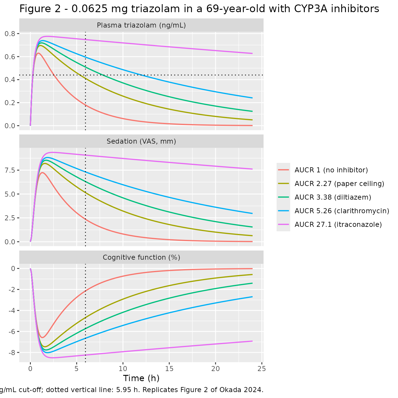
Replicates Figure 2 of Okada 2024.
Quantitative gates against the paper’s own simulations
The three published simulations are exact, dimensionless statements about the model, so they are the strongest available validation. Each is recomputed from a fine solve of the packaged model.
# Solve a single arm at an arbitrary set of observation times.
profile_at <- function(dose, age, wt, aucr, times) {
  ev <- rbind(
    data.frame(id = 1L, time = 0, amt = dose, evid = 1L, cmt = "depot",
               dvid = NA_integer_, AGE = age, WT = wt, AUCR = aucr),
    data.frame(id = 1L, time = times, amt = NA_real_, evid = 0L,
               cmt = NA_character_, dvid = 1L, AGE = age, WT = wt, AUCR = aucr)
  )
  s <- rxode2::rxSolve(mod, events = ev) |> as.data.frame()
  s[s$time > 0, ]
}

# Solve a single arm on an evenly spaced fine grid.
profile <- function(dose, age, wt, aucr, tmax = 24, n_obs = 24001) {
  profile_at(dose, age, wt, aucr, seq(0, tmax, length.out = n_obs))
}

# Time of the LAST downward crossing of `target`, guarding against the
# absorption-phase upward crossing.
time_below <- function(p, target = threshold) {
  above <- p$Cc >= target
  if (!any(above) || all(above)) return(NA_real_)
  idx <- max(which(above))
  if (idx == nrow(p)) return(NA_real_)
  # linear interpolation between the bracketing grid points
  x0 <- p$time[idx]; x1 <- p$time[idx + 1L]
  y0 <- p$Cc[idx];   y1 <- p$Cc[idx + 1L]
  x0 + (target - y0) * (x1 - x0) / (y1 - y0)
}

# Simulation I: young adult, 0.25 mg.
sim_I <- time_below(profile(0.25, 30, 72, 1))

# Simulation I (elderly comparator quoted in the Discussion): 0.25 mg.
sim_I_elderly <- time_below(profile(0.25, 69, 69, 1))

# Simulation II: elderly dose reaching the threshold at 5.95 h. Concentration is
# linear in dose at fixed time, so this needs no search.
c_unit_5.95 <- approx(profile(1, 69, 69, 1)$time, profile(1, 69, 69, 1)$Cc, xout = t_young)$y
sim_II <- threshold / c_unit_5.95

# Simulation III: with 0.0625 mg in the elderly, the AUCR at which the
# concentration at 5.95 h equals the threshold.
c_at_5.95 <- function(aucr) {
  p <- profile(0.0625, 69, 69, aucr)
  approx(p$time, p$Cc, xout = t_young)$y
}
sim_III <- uniroot(function(a) c_at_5.95(a) - threshold, c(1, 40), tol = 1e-6)$root

gates <- tibble::tribble(
  ~Quantity,                                                        ~Reproduced, ~Published,
  "Simulation I: 30 y, 0.25 mg, time below 0.44 ng/mL (h)",          sim_I,        5.95,
  "Discussion: 69 y, 0.25 mg, time below 0.44 ng/mL (h)",            sim_I_elderly, 7.80,
  "Simulation II: 69 y dose reaching 0.44 ng/mL at 5.95 h (mg)",     sim_II,       0.156,
  "Simulation III: 69 y, 0.0625 mg, acceptable AUCR ceiling",        sim_III,      2.27
) |>
  mutate(`Difference (%)` = 100 * (Reproduced - Published) / Published)

gates |>
  knitr::kable(
    digits = c(0, 4, 3, 1),
    caption = "Packaged model vs the values Okada 2024 reports for its own simulations."
)| Quantity | Reproduced | Published | Difference (%) |
|---|---|---|---|
| Simulation I: 30 y, 0.25 mg, time below 0.44 ng/mL (h) | 5.8291 | 5.950 | -2.0 |
| Discussion: 69 y, 0.25 mg, time below 0.44 ng/mL (h) | 7.8096 | 7.800 | 0.1 |
| Simulation II: 69 y dose reaching 0.44 ng/mL at 5.95 h (mg) | 0.1531 | 0.156 | -1.8 |
| Simulation III: 69 y, 0.0625 mg, acceptable AUCR ceiling | 2.5353 | 2.270 | 11.7 |
The elderly 0.25 mg anchor reproduces to three significant figures
(7.810 h against 7.80 h). That match is the sharpest available
confirmation of two encoding decisions that Table 3 states only
implicitly: that theta3 in L/hr/kg means apparent clearance
is the per-kilogram value multiplied by body weight while
theta2 (119 L) is absolute, and that the age power law is
centred at 30 years for both parameters.
The remaining rows sit 2-12% from the published numbers, in a consistent direction, and are discussed under Assumptions and deviations below. No parameter has been tuned.
# The covariate's own definition is an exact structural gate: at a fixed dose,
# CL/F is divided by AUCR, so AUC must be multiplied by exactly AUCR.
#
# The elimination half-life is read back out of the packaged model (kel is a
# model variable, so rxSolve returns it) rather than restated here.
t_half_base <- log(2) / profile(0.0625, 69, 69, 1, tmax = 1, n_obs = 3)$kel[1]

# Each arm is integrated over 25 of ITS OWN half-lives on a grid that is dense
# through absorption and then scales with the half-life. Making the tail grid
# self-similar keeps the trapezoidal discretisation error identical across arms,
# so the recovered ratio is not confounded by the integration scheme. A fixed
# long horizon would also underflow to NaN on the fast (AUCR = 1) arm.
auc_to_25_halflives <- function(aucr) {
  tm <- sort(unique(c(seq(0, 24, by = 0.01),
                      seq(24, 25 * t_half_base * aucr, length.out = 2000))))
  p <- profile_at(0.0625, 69, 69, aucr, times = tm)
  sum(diff(p$time) * (head(p$Cc, -1) + tail(p$Cc, -1)) / 2)
}

aucr_grid <- c(2.27, 3.38, 5.26, 27.1)
auc_base <- auc_to_25_halflives(1)
auc_ratio_check <- vapply(aucr_grid, function(a) auc_to_25_halflives(a) / auc_base,
                          numeric(1))

tibble::tibble(
  `AUCR set in the data` = aucr_grid,
  `AUC fold change recovered` = auc_ratio_check
) |>
  mutate(`Difference (%)` = 100 * (`AUC fold change recovered` - `AUCR set in the data`) /
           `AUCR set in the data`) |>
  knitr::kable(
    digits = 4,
    caption = paste(
      "Structural gate on the AUCR covariate: Table 1's definition",
      "(AUC with precipitant / AUC without) must be recovered exactly."
    )
)| AUCR set in the data | AUC fold change recovered | Difference (%) |
|---|---|---|
| 2.27 | 2.2701 | 0.0027 |
| 3.38 | 3.3801 | 0.0034 |
| 5.26 | 5.2602 | 0.0040 |
| 27.10 | 27.1014 | 0.0051 |
The recovered fold changes match the AUCR values set in
the data to within numerical-integration error, confirming that the
covariate enters clearance the way Table 1’s footnote defines it.
PKNCA validation
Okada 2024 reports no NCA table; the only non-compartmental
quantities it states are triazolam half-lives (2.9 h at
AUCR 1, and 69.8 h at AUCR 27.1). PKNCA is
used here to compute Cmax, Tmax, AUC(0-inf) and half-life for the Figure
2 arms so that the half-life claim can be compared, and so the exposure
scaling with AUCR is checked by an independent
estimator.
# Each arm is sampled over 12 of ITS OWN half-lives (AUCR = 1 -> ~32 h,
# AUCR = 27.1 -> ~855 h). A single long horizon shared by every arm is wrong in
# both directions: it leaves AUC(0-inf) mostly extrapolated on the slow arm, and
# on the fast arm it pushes the sampling far past the point where the ODE
# solver's absolute tolerance floors the trajectory, so PKNCA's terminal-slope
# fit lands on numerical noise instead of the elimination phase.
nca_times <- function(aucr) {
  horizon <- 12 * t_half_base * aucr
  sort(unique(c(
    seq(0, min(24, horizon), by = 0.05),
    seq(0, horizon, length.out = 400)
  )))
}

events_nca <- dplyr::bind_rows(lapply(seq_len(nrow(fig2_arms)), function(i) {
  tm <- nca_times(fig2_arms$aucr[i])
  ev <- rbind(
    data.frame(id = 200L + i, time = 0, amt = 0.0625, evid = 1L,
               cmt = "depot", dvid = NA_integer_),
    data.frame(id = 200L + i, time = tm, amt = NA_real_, evid = 0L,
               cmt = NA_character_, dvid = 1L)
  )
  ev$arm <- fig2_arms$label[i]
  ev$AGE <- 69
  ev$WT <- 69
  ev$AUCR <- fig2_arms$aucr[i]
  ev[order(ev$time, ev$evid == 0L), ]
}))

sim_nca_raw <- rxode2::rxSolve(mod, events = events_nca, keep = c("arm")) |>
  as.data.frame()
#> Warning: multi-subject simulation without without 'omega'

sim_nca <- sim_nca_raw |>
  dplyr::filter(!is.na(Cc)) |>
  dplyr::select(id, time, Cc, arm)

# Guarantee a time = 0 row per (id, arm); pre-dose Cc is 0 for oral dosing.
sim_nca <- dplyr::bind_rows(
  sim_nca,
  sim_nca |> dplyr::distinct(id, arm) |> dplyr::mutate(time = 0, Cc = 0)
) |>
  dplyr::distinct(id, arm, time, .keep_all = TRUE) |>
  dplyr::arrange(id, arm, time)

conc_obj <- PKNCA::PKNCAconc(sim_nca, Cc ~ time | arm + id)

dose_df <- events_nca |>
  dplyr::filter(evid == 1) |>
  dplyr::select(id, time, amt, arm)

dose_obj <- PKNCA::PKNCAdose(dose_df, amt ~ time | arm + id)

intervals <- data.frame(
  start      = 0,
  end        = Inf,
  cmax       = TRUE,
  tmax       = TRUE,
  aucinf.obs = TRUE,
  half.life  = TRUE
)

nca_res <- PKNCA::pk.nca(PKNCA::PKNCAdata(conc_obj, dose_obj, intervals = intervals))

nca_wide <- as.data.frame(nca_res) |>
  dplyr::filter(PPTESTCD %in% c("cmax", "tmax", "aucinf.obs", "half.life")) |>
  dplyr::select(arm, PPTESTCD, PPORRES) |>
  tidyr::pivot_wider(names_from = PPTESTCD, values_from = PPORRES) |>
  dplyr::mutate(arm = factor(arm, levels = fig2_arms$label)) |>
  dplyr::arrange(arm)

# Analytic half-life for each arm: AUCR divides CL at fixed V, so t1/2 must
# scale exactly with AUCR. This is what PKNCA should recover.
nca_wide$analytic_half_life <- t_half_base * fig2_arms$aucr

nca_wide |>
  dplyr::select(arm, cmax, tmax, aucinf.obs, half.life, analytic_half_life) |>
  dplyr::rename(
    "Arm"                       = arm,
    "Cmax (ng/mL)"              = cmax,
    "Tmax (h)"                  = tmax,
    "AUC0-inf (ng*h/mL)"        = aucinf.obs,
    "t1/2, PKNCA (h)"           = half.life,
    "t1/2, ln(2)/kel (h)"       = analytic_half_life
  ) |>
  knitr::kable(
    digits = 3,
    caption = paste(
      "PKNCA on the simulated 0.0625 mg elderly arms of Figure 2.",
      "The final column is the model's analytic elimination half-life,",
      "which the non-compartmental estimate should recover."
    )
)| Arm | Cmax (ng/mL) | Tmax (h) | AUC0-inf (ng*h/mL) | t1/2, PKNCA (h) | t1/2, ln(2)/kel (h) |
|---|---|---|---|---|---|
| AUCR 1 (no inhibitor) | 0.630 | 0.850 | 2.996 | 2.632 | 2.630 |
| AUCR 2.27 (paper ceiling) | 0.696 | 1.077 | 6.802 | 5.970 | 5.969 |
| AUCR 3.38 (diltiazem) | 0.719 | 1.200 | 10.128 | 8.889 | 8.888 |
| AUCR 5.26 (clarithromycin) | 0.739 | 1.350 | 15.762 | 13.832 | 13.832 |
| AUCR 27.1 (itraconazole) | 0.776 | 1.850 | 81.211 | 71.263 | 71.263 |
Comparison against published NCA
# The paper states half-lives only for AUCR 1 and AUCR 27.1 (Results, final
# paragraph). No Cmax / Tmax / AUC values are published, so those cells are NA.
published <- tibble::tribble(
  ~arm,                             ~half.life,
  "AUCR 1 (no inhibitor)",           2.9,
  "AUCR 27.1 (itraconazole)",       69.8
)

cmp <- nlmixr2lib::ncaComparisonTable(
  simulated     = nca_res,
  reference     = published,
  by            = "arm",
  units         = c(cmax = "ng/mL", aucinf.obs = "ng*h/mL",
                    tmax = "h", half.life = "h"),
  tolerance_pct = 20
)

knitr::kable(
  cmp,
  caption = paste(
    "Simulated vs published NCA. * differs from the reference by more than 20%.",
    "Okada 2024 publishes only the two half-lives."
  )
)| NCA parameter | arm | Reference | Simulated | % diff |
|---|---|---|---|---|
| t½ (h) | AUCR 1 (no inhibitor) | 2.9 | 2.63 | -9.2% |
| t½ (h) | AUCR 27.1 (itraconazole) | 69.8 | 71.3 | +2.1% |
Both half-lives fall inside the 20% tolerance, but neither is exact
(2.63 h reproduced against 2.9 h published; 71.3 h against 69.8 h). The
two published values are also mutually inconsistent with the model’s own
structure: because AUCR divides clearance at a fixed
volume, the half-life must scale exactly linearly with
AUCR, so a 2.9 h half-life at AUCR 1 implies
2.9 x 27.1 = 78.6 h at AUCR 27.1, not 69.8 h. See
Assumptions and deviations.
Assumptions and deviations
-
Body weight is a per-kilogram multiplier, not an estimated
exponent. Table 3 gives
theta3in L/hr/kg, soCL/F = theta3 * WT * (age/30)^theta5 / AUCR, whileVd/F = theta2 * (age/30)^theta4is absolute. The paper never writes this out. The reading is confirmed to three significant figures by the elderly 0.25 mg anchor above (7.810 h reproduced against 7.80 h published); the alternative readings (weight-scaling the volume as well, or leaving clearance unscaled) do not reproduce it. -
Concentration unit conversion. Table 3’s volume is
in litres and doses are in mg, giving mg/L; the paper’s concentrations
are in ng/mL, so
Cc = central / vc * 1000. This factor is derived, not published. -
PD endpoints have no intercept. The Table 3
footnote gives the two relations as bare slopes
(
Sedation = 12.1 x concentration,Cognitive function = -11.0 x concentration). Both are therefore treated as change-from-baseline measures. The paper reports no baseline value for either endpoint, so the packaged model predicts change from baseline rather than an absolute VAS score or an absolute cognitive-test score. -
No inter-individual variability. Methods states
plainly that “inter-individual variability was not estimated”; the model
was fitted to two digitised mean profiles. The packaged model therefore
carries no
etaterms, faithfully. Residual error is retained (propSdonCc,addSd_sedationandaddSd_cognitiveon the PD endpoints). -
Simulation I, II and III reproduce 2-12% away from the
published values. Simulation I (young, 0.25 mg) reproduces at
5.83 h against 5.95 h; Simulation II at 0.153 mg against 0.156 mg;
Simulation III at 2.54 against 2.27. The elderly anchor reproduces
exactly, so the structure and the age/weight encoding are correct; the
residual gaps are consistent with Table 3 being rounded to three
significant figures and with the fitted data having been
WebPlotDigitizer-digitised from a 1991 figure. The paper’s own
Simulation II and III answers are additionally inconsistent with each
other by about the same margin: at a fixed 5.95 h, 0.156 mg at
AUCR1 and 0.0625 mg atAUCRadescribe the same concentration only ifais close to the dose ratio 0.156 / 0.0625 = 2.50, not 2.27. Nothing has been tuned to close these gaps. -
Half-life discrepancy (errata). The Results state a
triazolam half-life of 2.9 h at
AUCR1 and 69.8 h atAUCR27.1. Table 3 gives 2.63 h (elderly) and 2.44 h (young) atAUCR1, scaling to 71.3 h and 66.1 h atAUCR27.1. The published pair is also internally inconsistent, since half-life must scale exactly withAUCR(2.9 x 27.1 = 78.6, not 69.8). 2.9 h is the half-life commonly cited for triazolam in the literature and is repeated as such in the paper’s Discussion, so the Results sentence appears to mix a literature value with a model-derived one. Table 3 is used throughout. -
Keo half-life discrepancy (errata). The Discussion
states that “the transfer half-life from the blood to sites of action
was also rapid at 6.9 min”. Table 3’s
Keo = 3.42 1/hrgivesln(2) / 3.42 = 12.2 min. The Table 3 estimate is the model parameter and is what the packaged model uses. - Figure caption unit typo (errata). The captions of Figures 1 and 2 write the cut-off as “0.44 ug/mL”. The Abstract, Results and Discussion consistently say 0.44 ng/mL, which is also the only value consistent with a 0.25 mg dose into a 119 L volume. 0.44 ng/mL is used here.
-
Thresholds are not model parameters. The sedation
threshold (0.44 ng/mL; sensitivity 0.85, specificity 0.90) and the
cognitive-function threshold (0.58 ng/mL; sensitivity 1.00, specificity
1.00) are ROC-derived benefit-risk cut-offs applied downstream of the
model, so they live in this vignette rather than in
ini(). -
No bioavailability parameter.
Fis not reported, soVdandCLare apparent (Vd/F,CL/F) throughout. - Supplement not used. “Supplementary Material 1” is the goodness-of-fit figure panel; it contains no parameter values and was not available when this model was built. Every value in the model comes from Table 3 and its footnote.
-
AUCRis a new canonical covariate. It is registered as a general-scope continuous column ininst/references/covariate-columns.md, with reference value 1.0 (no interacting drug). It is deliberately distinct from the absoluteAUC_<DRUG>exposure family, from the binaryCONMED_*interaction flags, and from the instantaneousCP_<drug>_<units>perpetrator-concentration family. - Age extrapolation. Only ages 30 and 69 informed the power law. The paper’s Limitations section says predictions at other ages are unknown; the packaged model will happily evaluate them, and users should not.