Acalabrutinib and ACP-5862 (Edlund 2022)
Source:vignettes/articles/Edlund_2022_acalabrutinib.Rmd
Edlund_2022_acalabrutinib.RmdModel and source
- Citation: Edlund H, Bellanti F, Liu H, Vishwanathan K, Tomkinson H, Ware J, Sharma S, Buil-Bruna N. Improved characterization of the pharmacokinetics of acalabrutinib and its pharmacologically active metabolite, ACP-5862, in patients with B-cell malignancies and in healthy subjects using a population pharmacokinetic approach. Br J Clin Pharmacol. 2022;88(2):846-852. doi:10.1111/bcp.14988
- Description: Joint parent-metabolite population PK model for oral acalabrutinib and its active metabolite ACP-5862 in adults with B-cell malignancies and healthy subjects (Edlund 2022). Acalabrutinib: two-compartment disposition with first-order elimination; absorption through a dosing depot, a chain of five transit compartments and an absorption depot (mean transit time MTT = (Ntr + 1) / ktr) followed by first-order absorption, with between-occasion variability on MTT and on the relative bioavailability F1. ACP-5862: two-compartment disposition with first-order elimination, formed at 0.4 x CL/F (fraction metabolised held at 0.4 from the human ADME study). Healthy-subject status acts on CL/F and Vp/F, ECOG performance status >= 2 on CL/F, and concomitant proton-pump-inhibitor use on F1. Separate log-scale residual errors for each analyte on rich-profile versus sparse sampling occasions.
- Article: https://doi.org/10.1111/bcp.14988 (open access; the Supporting Information document BCP-88-846-s001 holds the study table, the demographics, the covariate equations and the final-model schematic, Figure S10)
Edlund 2022 updates an earlier acalabrutinib / ACP-5862 population PK
model (Edlund 2019, Clin Pharmacokinet 58:659-672) with substantially
more patient data. The model is a joint parent-metabolite model:
acalabrutinib is absorbed through a dosing depot, five transit
compartments and an absorption depot, distributes into two compartments,
and is cleared at CL/F, of which the fraction fm = 0.4
forms ACP-5862, which itself has two-compartment disposition.
Population
The analysis pooled 12 studies (Supplement Table S1): four phase 1 studies in 138 healthy subjects (single 75 or 100 mg doses, including two drug-drug interaction studies with omeprazole) and eight phase 1-3 studies in 575 patients with B-cell malignancies (100-400 mg QD or 100-200 mg BID). The dataset held 8935 acalabrutinib samples from 712 subjects and 2394 ACP-5862 samples from 304 subjects. Patients were older than the healthy subjects (mean 66.9 vs 42.0 years) and similar in body weight (overall mean 81.0 kg, range 39.9-148.6); 33.2% were female and 89.6% White (Tables S2-S3). Chronic lymphocytic leukaemia was the dominant indication (443 of 575 patients), followed by Waldenstrom macroglobulinaemia, mantle cell lymphoma, diffuse large B-cell lymphoma, multiple myeloma and follicular lymphoma. 27 patients had ECOG performance status 2 or 3 and 66 used a proton-pump inhibitor (PPI).
The same information is available programmatically via
readModelDb("Edlund_2022_acalabrutinib")()$population.
Source trace
Every ini() value carries an in-file comment pointing at
its source. The table collects them.
| Equation / parameter | Value | Source location |
|---|---|---|
lcl (CL/F) |
log(134) L/h | Table 1 |
lvc (Vc/F) |
log(31.0) L | Table 1 |
lq (Q/F) |
log(20.9) L/h | Table 1 |
lvp (Vp/F) |
log(110) L | Table 1 |
lka (Ka) |
log(1.48) 1/h | Table 1 |
lmtt (MTT) |
log(0.459) h | Table 1 |
ntr |
5 (not estimated) | Results 3.2, Figure S10 |
lfdepot (F1) |
log(1) (reference) | Results 3.2 (relative F1 with BOV); no F1 row in Table 1 |
fm |
0.4 (not estimated) | Methods 2.2 (human ADME study) |
lcl_acp (CLM/F) |
log(21.8) L/h | Table 1 |
lvc_acp (VcM/F) |
log(22.7) L | Table 1 |
lq_acp (QM/F) |
log(26.7) L/h | Table 1 |
lvp_acp (VpM/F) |
log(89.2) L | Table 1 |
e_dis_healthy_cl |
0.467 | Table 1; sign from Supplement Discussion (196 L/h in healthy subjects) |
e_dis_healthy_vp |
-0.556 | Table 1; sign from Supplement Discussion (49 L in healthy subjects) |
e_ecog_ge2_cl |
-0.171 | Table 1; sign from Discussion (+21% AUC with ECOG >= 2) |
e_conmed_ppi_fdepot |
-0.358 | Table 1; sign from Results 3.3 (-36% AUC with PPI) |
etalcl, etalvc, etalvp
|
0.0551, 2.12, 0.108 | Table 1 BSV 23.8, 270, 33.7 CV% |
etalcl_acp, etalvc_acp,
etalq_acp, etalvp_acp
|
0.0138, 0.201, 0.153, 0.0362 | Table 1 BSV 11.8, 47.2, 40.7, 19.2 CV% |
etaiov_mtt_1..4 |
0.872 | Table 1 BOV MTT 118 CV%; 4 occasions (footnote b) |
etaiov_fdepot_1..4 |
0.274 | Table 1 BOV F1 56.1 CV% |
expSdIntensive, expSdSparse
|
0.586, 0.856 | Table 1 residual error (SD), rich and sparse |
expSdIntensive_acp, expSdSparse_acp
|
0.334, 0.234 | Table 1 metabolite residual error (SD), rich and sparse |
Covariate form theta * (1 + theta_cov)^cov
|
n/a | Supplement Eq. 2; Table 1 footnote c |
Transit chain, absorption depot,
ktr = (ntr + 1) / mtt
|
n/a | Figure S10 and its legend |
Formation fm * CL/F * Cp into ACP-5862 central |
n/a | Methods 2.2, Results 3.2, Figure S10 |
Molar conversion mw_acp / mw_parent = 481.52 /
465.52 |
n/a | Molecular formulae; Supplement LLOQ pairs 1.0 ng/mL = 2.1 nM, 5 ng/mL = 10.4 nM |
| Log-scale (exponential) residual error | n/a | Methods 2.2, Results 3.2 |
Simulation design
The paper’s exposure metrics (Results 3.3 and Supplement “Acalabrutinib and ACP-5862 exposures”) were generated by simulating 14 days at steady state in which each dose drew its own F1 and MTT from the between-occasion distributions; AUC24h,ss was the cumulative 14-day AUC divided by 14 and Cmax,ss the average of the per-dose Cmax values. The reference population is a patient with ECOG performance status 0-1 and no PPI at 100 mg BID.
The packaged model carries four occasion slots (the analysis’s three
rich occasions plus the lumped sparse occasion, selected by
OCC). To reproduce a fresh draw at every dose, the vignette
keeps every record on OCC = 1 and supplies
etaiov_mtt_1 / etaiov_fdepot_1 as columns of
the event table whose value changes at each dose. All random effects are
drawn in R and passed on the event rows with omega = NA, so
the cohort is identical on every machine, and the same draws are reused
across the covariate arms (common random numbers).
mod <- readModelDb("Edlund_2022_acalabrutinib")
ui <- rxode2::rxode2(mod)
#> ℹ parameter labels from comments will be replaced by 'label()'
#> Warning: some etas defaulted to non-mu referenced, possible parsing error: etaiov_mtt_1, etaiov_mtt_2, etaiov_mtt_3, etaiov_mtt_4, etaiov_fdepot_1, etaiov_fdepot_2, etaiov_fdepot_3, etaiov_fdepot_4
#> as a work-around try putting the mu-referenced expression on a simple line
om <- ui$omega

n_sub <- 200
tau <- 12
n_run_in <- 6 # three days of BID dosing to reach steady state
n_window <- 28 # the paper's 14-day steady-state window
t_win <- c(n_run_in * tau, (n_run_in + n_window) * tau)
dose_times <- (seq_len(n_run_in + n_window + 1) - 1) * tau

set.seed(20220211)
# Between-subject etas: Latin-hypercube quantiles so every marginal is
# reproduced exactly at n = 200 while the etas stay mutually independent.
lhs <- function(v) sqrt(v) * qnorm((sample.int(n_sub) - 0.5) / n_sub)
bsv_names <- c("etalcl", "etalvc", "etalvp", "etalcl_acp", "etalvc_acp",
               "etalq_acp", "etalvp_acp")
subj <- tibble(id = seq_len(n_sub))
for (nm in bsv_names) subj[[nm]] <- lhs(om[nm, nm])

# One BOV draw per dose and subject.
dose_iov <- expand.grid(dose_k = seq_along(dose_times), id = seq_len(n_sub)) |>
  as_tibble() |>
  mutate(
    time = dose_times[dose_k],
    etaiov_mtt_1 = rnorm(n(), 0, sqrt(om["etaiov_mtt_1", "etaiov_mtt_1"])),
    etaiov_fdepot_1 = rnorm(n(), 0, sqrt(om["etaiov_fdepot_1", "etaiov_fdepot_1"]))
  )

# Dense (0.1 h) over the first 4 h after each dose, where the peak lies,
# 0.5 h over the rest of the interval.
tad_grid <- c(seq(0, 4, by = 0.1), seq(4.5, tau - 0.5, by = 0.5))
obs_times <- c(as.vector(outer(tad_grid, seq(t_win[1], t_win[2] - tau, by = tau), "+")),
               t_win[2])

make_arm <- function(arm, healthy, ecog2, ppi, id_offset) {
  doses <- dose_iov |>
    mutate(evid = 1L, amt = 100, cmt = "depot", dvid = NA_integer_)
  obs <- expand.grid(time = obs_times, id = seq_len(n_sub)) |>
    as_tibble() |>
    mutate(evid = 0L, amt = 0, cmt = "central", dvid = 1L)
  bind_rows(doses, obs) |>
    arrange(id, time, desc(evid)) |>
    group_by(id) |>
    tidyr::fill(dose_k, etaiov_mtt_1, etaiov_fdepot_1) |>
    ungroup() |>
    left_join(subj, by = "id") |>
    mutate(
      id = id + id_offset, arm = arm, OCC = 1L, SAMPLE_INTENSIVE = 1L,
      # copy of the F1 draw under a non-parameter name, carried through `keep`
      f_eta = etaiov_fdepot_1,
      DIS_HEALTHY = healthy, ECOG_GE2 = ecog2, CONMED_PPI = ppi
    )
}

arms <- tribble(
  ~arm,             ~healthy, ~ecog2, ~ppi,
  "Reference",      0L,       0L,     0L,
  "Healthy",        1L,       0L,     0L,
  "ECOG >= 2",      0L,       1L,     0L,
  "PPI",            0L,       0L,     1L
)
events <- bind_rows(lapply(seq_len(nrow(arms)), function(i) {
  make_arm(arms$arm[i], arms$healthy[i], arms$ecog2[i], arms$ppi[i],
           id_offset = (i - 1L) * n_sub)
}))
stopifnot(!anyDuplicated(events[, c("id", "time", "evid")]))
sim <- suppressWarnings(rxode2::rxSolve(
  mod, events = events, omega = NA, returnType = "data.frame",
  keep = c("arm", "dose_k", "f_eta"), addDosing = FALSE
))
#> ℹ parameter labels from comments will be replaced by 'label()'
sim <- sim |> mutate(arm = factor(arm, levels = arms$arm))

# Harness check: the per-dose BOV and the per-subject BSV supplied on the
# event rows must actually reach the model. If eta columns were silently
# ignored, fdepot would be 1 and cl would be 134 L/h for everyone.
chk <- sim |> filter(arm == "Reference")
stopifnot(
  max(abs(chk$fdepot / exp(chk$f_eta) - 1)) < 1e-8,
  sd(log(chk$fdepot)) > 0.3
)
# rxSolve returns the supplied eta columns alongside the model variables.
cl_chk <- sim |>
  group_by(id) |>
  slice(1) |>
  ungroup()
stopifnot(all(abs(cl_chk$etalcl -
  subj$etalcl[(cl_chk$id - 1L) %% n_sub + 1L]) < 1e-12))
stopifnot(max(abs(cl_chk$cl / (134 * exp(cl_chk$etalcl) *
  1.467^(cl_chk$arm == "Healthy") * 0.829^(cl_chk$arm == "ECOG >= 2")) - 1)) < 1e-8)
Typical-value profiles
A single 100 mg dose for a typical patient and a typical healthy subject, all random effects at zero. ACP-5862 peaks later than acalabrutinib and declines more slowly, so it dominates the plasma exposure.
ev_typ <- bind_rows(
  tibble(id = 1L, time = 0, amt = 100, evid = 1L, cmt = "depot", dvid = NA_integer_),
  tibble(id = 1L, time = seq(0, 24, by = 0.05), amt = 0, evid = 0L,
         cmt = "central", dvid = 1L)
)
ev_typ <- bind_rows(
  ev_typ |> mutate(DIS_HEALTHY = 0L, group = "Patient"),
  ev_typ |> mutate(id = 2L, DIS_HEALTHY = 1L, group = "Healthy subject")
) |>
  mutate(ECOG_GE2 = 0L, CONMED_PPI = 0L, OCC = 1L, SAMPLE_INTENSIVE = 1L)
sim_typ <- suppressWarnings(rxode2::rxSolve(
  mod, events = ev_typ, omega = NA, returnType = "data.frame",
  keep = "group", addDosing = FALSE
))

sim_typ |>
  select(time, group, Acalabrutinib = Cc, `ACP-5862` = Cc_acp) |>
  pivot_longer(c(Acalabrutinib, `ACP-5862`), names_to = "analyte", values_to = "conc") |>
  ggplot(aes(time, conc, colour = group)) +
  geom_line() +
  facet_wrap(~analyte) +
  scale_y_log10(limits = c(0.5, NA)) +
  labs(x = "Time after a single 100 mg dose (h)", y = "Concentration (ng/mL)",
       colour = NULL, caption = "Typical-value prediction, random effects at zero.")
#> Warning in scale_y_log10(limits = c(0.5, NA)): log-10 transformation introduced
#> infinite values.
#> Warning: Removed 282 rows containing missing values or values outside the scale range
#> (`geom_line()`).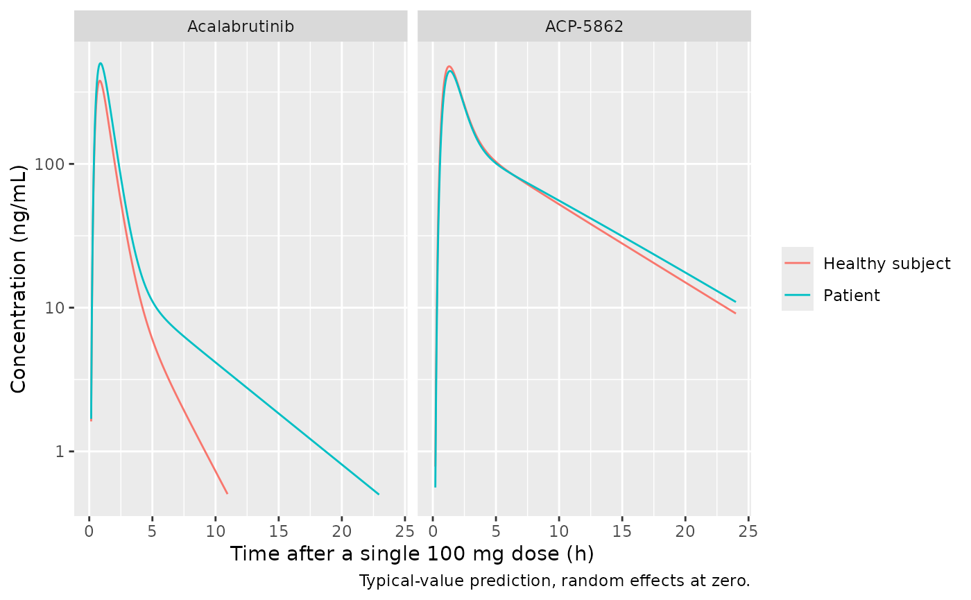
Steady-state 12-hour profile
Percentiles of the simulated 100 mg BID steady-state profile over all 28 dosing intervals of the window, for the reference population. This mirrors the 12-hour layout of the paper’s pcVPC (Figure 1), which shows only prediction-corrected percentiles and no published numbers to compare against.
sim |>
  filter(arm == "Reference") |>
  mutate(tad = time - t_win[1] - (dose_k - n_run_in - 1) * tau) |>
  filter(tad < tau) |>
  mutate(tad = round(tad, 1)) |>
  select(tad, Acalabrutinib = Cc, `ACP-5862` = Cc_acp) |>
  pivot_longer(-tad, names_to = "analyte", values_to = "conc") |>
  group_by(analyte, tad) |>
  summarise(
    p10 = quantile(conc, 0.1), p50 = median(conc), p90 = quantile(conc, 0.9),
    .groups = "drop"
  ) |>
  ggplot(aes(tad, p50)) +
  geom_ribbon(aes(ymin = p10, ymax = p90), alpha = 0.25) +
  geom_line() +
  facet_wrap(~analyte, scales = "free_y") +
  scale_y_log10() +
  labs(x = "Time after dose (h)", y = "Concentration (ng/mL)",
       caption = paste("Median and 10th-90th percentiles; reference population,",
                       "100 mg BID at steady state. Layout of Figure 1 of Edlund 2022."))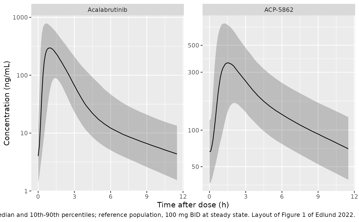
PKNCA validation
AUC24h,ss is the paper’s cumulative 14-day steady-state AUC divided by 14. PKNCA computes the AUC over the whole 14-day window (one interval per subject, analyte and arm) from the simulated profile, sampled every 0.25 h over the first 2 h after each dose and every 0.5 h otherwise. Cmax,ss is the mean of the 28 per-dose maxima, taken from the simulation grid (0.1 h over the first 4 h after each dose). Running PKNCA on each of the 28 dosing intervals separately gives the same AUC but costs about 45,000 PKNCA intervals across the four arms, too slow for this article.
conc_long <- sim |>
  filter(!is.na(Cc)) |>
  select(id, time, dose_k, arm, Acalabrutinib = Cc, `ACP-5862` = Cc_acp) |>
  pivot_longer(c(Acalabrutinib, `ACP-5862`), names_to = "analyte", values_to = "Cc") |>
  mutate(treatment = paste(arm, analyte, sep = " | "))

# PKNCA input: every 0.25 h over the first 2 h after each dose, which holds
# the peak, and every 0.5 h over the rest of the interval.
conc_nca <- conc_long |>
  mutate(tad = (time - t_win[1]) %% tau) |>
  filter(abs(time * 2 - round(time * 2)) < 1e-6 |
    (tad < 2 + 1e-6 & abs(time * 4 - round(time * 4)) < 1e-6)) |>
  select(id, time, Cc, treatment)
stopifnot(all(conc_nca |> group_by(id, treatment) |>
  summarise(t0 = min(time), t1 = max(time), .groups = "drop") |>
  with(t0 == t_win[1] & t1 == t_win[2])))

dose_df <- events |>
  filter(evid == 1, time >= t_win[1], time < t_win[2]) |>
  select(id, time, amt, arm) |>
  tidyr::crossing(analyte = c("Acalabrutinib", "ACP-5862")) |>
  mutate(treatment = paste(arm, analyte, sep = " | ")) |>
  select(-arm, -analyte)

intervals <- data.frame(start = t_win[1], end = t_win[2], auclast = TRUE)
# One PKNCA call per arm and analyte: PKNCA's run time grows faster than
# linearly with the number of subjects in one call, and eight calls of 200
# subjects run several times faster than a single call of 1600.
nca_one <- function(trt) {
  conc_obj <- PKNCA::PKNCAconc(filter(conc_nca, treatment == trt), Cc ~ time | treatment + id)
  dose_obj <- PKNCA::PKNCAdose(filter(dose_df, treatment == trt), amt ~ time | treatment + id)
  res <- PKNCA::pk.nca(PKNCA::PKNCAdata(conc_obj, dose_obj, intervals = intervals))
  as.data.frame(res$result)
}
nca_res <- bind_rows(lapply(unique(conc_nca$treatment), nca_one))

auc_ss <- nca_res |>
  filter(PPTESTCD == "auclast") |>
  transmute(treatment, id, PPTESTCD = "auc24ss", value = PPORRES / 14)
cmax_ss <- conc_long |>
  filter(time < t_win[2]) |>
  group_by(treatment, id, dose_k) |>
  summarise(cmax = max(Cc), .groups = "drop_last") |>
  summarise(value = mean(cmax), n_int = n(), .groups = "drop") |>
  mutate(PPTESTCD = "cmaxss")
stopifnot(all(cmax_ss$n_int == n_window))
ss <- bind_rows(auc_ss, select(cmax_ss, -n_int)) |>
  separate(treatment, c("arm", "analyte"), sep = " \\| ")
stopifnot(nrow(ss) == n_sub * 4 * 2 * 2, !anyNA(ss$value))
Comparison against the published reference-population exposures
Results 3.3 reports the model-predicted median (90% prediction interval) for the reference population at 100 mg BID.
published <- tribble(
  ~analyte,        ~PPTESTCD,  ~p50,   ~p05,   ~p95,
  "Acalabrutinib", "auc24ss",  1668,   1094,   2536,
  "Acalabrutinib", "cmaxss",   461,    199.8,  783.3,
  "ACP-5862",      "auc24ss",  4175,   3256,   5430,
  "ACP-5862",      "cmaxss",   461.3,  263.7,  678.4
)
ref_sim <- ss |> filter(arm == "Reference")

# auc24ss / cmaxss are not PKNCA codes (they are the paper's 14-day
# averages), so the helper keeps the codes as labels; relabel them here.
cmp <- suppressWarnings(nlmixr2lib::ncaComparisonTable(
  simulated = ref_sim |> transmute(analyte, PPTESTCD, PPORRES = value),
  reference = published |> select(analyte, PPTESTCD, PPORRES = p50),
  by = "analyte",
  units = c(auc24ss = "ng*h/mL", cmaxss = "ng/mL"),
  tolerance_pct = 20
))
cmp[[1]] <- sub("^cmaxss", "Cmax,ss", sub("^auc24ss", "AUC24h,ss", cmp[[1]]))
stopifnot(nrow(cmp) == 4, !any(grepl("auc24ss|cmaxss", cmp[[1]])))
knitr::kable(cmp, caption = paste(
  "Median simulated vs published exposures, reference population, 100 mg BID.",
  "* differs from the reference by > 20%."
))| NCA parameter | analyte | Reference | Simulated | % diff |
|---|---|---|---|---|
| AUC24h,ss (ng*h/mL) | Acalabrutinib | 1670 | 1710 | +2.3% |
| AUC24h,ss (ng*h/mL) | ACP-5862 | 4180 | 4320 | +3.5% |
| Cmax,ss (ng/mL) | Acalabrutinib | 461 | 491 | +6.5% |
| Cmax,ss (ng/mL) | ACP-5862 | 461 | 505 | +9.4% |
pi_tab <- ref_sim |>
  group_by(analyte, PPTESTCD) |>
  summarise(sim_p05 = quantile(value, 0.05), sim_p50 = median(value),
            sim_p95 = quantile(value, 0.95), .groups = "drop") |>
  left_join(published, by = c("analyte", "PPTESTCD")) |>
  mutate(across(c(sim_p05, sim_p95), \(x) round(x, 1)),
         pct_p05 = round(100 * (sim_p05 / p05 - 1), 1),
         pct_p50 = round(100 * (sim_p50 / p50 - 1), 1),
         pct_p95 = round(100 * (sim_p95 / p95 - 1), 1))
pi_tab |>
  select(analyte, PPTESTCD, p05, sim_p05, pct_p05, p95, sim_p95, pct_p95) |>
  rename(
    "Analyte" = analyte, "Metric" = PPTESTCD,
    "Published 5th" = p05, "Simulated 5th" = sim_p05, "% diff 5th" = pct_p05,
    "Published 95th" = p95, "Simulated 95th" = sim_p95, "% diff 95th" = pct_p95
  ) |>
knitr::kable(caption = "Bounds of the 90% prediction interval, simulated vs published.")| Analyte | Metric | Published 5th | Simulated 5th | % diff 5th | Published 95th | Simulated 95th | % diff 95th |
|---|---|---|---|---|---|---|---|
| ACP-5862 | auc24ss | 3256.0 | 3388.3 | 4.1 | 5430.0 | 5411.0 | -0.3 |
| ACP-5862 | cmaxss | 263.7 | 281.1 | 6.6 | 678.4 | 716.3 | 5.6 |
| Acalabrutinib | auc24ss | 1094.0 | 1122.3 | 2.6 | 2536.0 | 2530.7 | -0.2 |
| Acalabrutinib | cmaxss | 199.8 | 205.9 | 3.1 | 783.3 | 800.4 | 2.2 |
# The cohort is drawn in R and passed with omega = NA, so it is identical on
# every machine. Realised median offsets: AUC +2.3% / +3.5%, Cmax +6.5% /
# +9.4% (acalabrutinib / ACP-5862). Structural: a mis-transcribed clearance,
# volume, fm, molar factor or BOV variance moves these medians by tens of
# percent. Envelope: the 90% PI
# bounds carry the BSV / BOV magnitudes (reading the Table 1 CV% as the
# variance itself would put the parent Cmax,ss 5th percentile near 85 ng/mL,
# more than 50% below the published 199.8).
stopifnot(
  all(abs(pi_tab$pct_p50) < 12),
  all(abs(pi_tab$pct_p05) < 20),
  all(abs(pi_tab$pct_p95) < 20)
)
The simulated medians sit above the published ones: by 2-4% for AUC24h,ss and by 7-9% for Cmax,ss, for both analytes. The AUC offset is common to acalabrutinib and ACP-5862, as expected when the two share the per-dose F1 draws, and the ratio of the ACP-5862 to the acalabrutinib median AUC (published 4175 / 1668 = 2.50) is reproduced to within about 1%, which supports the molar conversion of the formation flux. The slightly larger Cmax offset is consistent with the 0.1 h output grid used here resolving the narrow absorption peak better than a coarser simulation grid would; the paper does not state its grid. The prediction-interval bounds agree to within 7%. No published parameter was changed to close these gaps.
Closed-form check on the simulated AUC
For a linear model, the steady-state AUC over the window equals the
dose delivered in the window divided by clearance. Per subject,
AUC24h,ss for acalabrutinib is therefore
2 * 100 mg * mean(F1) / CL * 1000, and for ACP-5862
fm * (MW_ACP / MW_acalabrutinib) * 2 * 100 mg * mean(F1) / CLM * 1000,
with mean(F1) taken over the doses of the window. Both
sides use the same drawn parameters, so the difference is trapezoidal
and window-edge error only.
f_win <- events |>
  filter(evid == 1, time >= t_win[1], time < t_win[2]) |>
  group_by(id) |>
  summarise(mean_f = mean(exp(etaiov_fdepot_1) * 0.642^CONMED_PPI), .groups = "drop")
par_i <- sim |>
  group_by(id) |>
  slice(1) |>
  ungroup() |>
  select(id, arm, cl, cl_acp) |>
  left_join(f_win, by = "id") |>
  mutate(arm = as.character(arm))
cf <- ss |>
  filter(PPTESTCD == "auc24ss") |>
  left_join(par_i, by = c("id", "arm")) |>
  mutate(
    expected = ifelse(analyte == "Acalabrutinib",
                      2 * 100 * mean_f / cl * 1000,
                      0.4 * (481.52 / 465.52) * 2 * 100 * mean_f / cl_acp * 1000),
    pct_diff = 100 * (value / expected - 1)
  )
cf |>
  group_by(analyte) |>
  summarise(median_pct = median(pct_diff), q90_abs_pct = quantile(abs(pct_diff), 0.9)) |>
knitr::kable(digits = 2, caption = "Simulated vs closed-form AUC24h,ss, all arms.")| analyte | median_pct | q90_abs_pct |
|---|---|---|
| ACP-5862 | -0.02 | 1.19 |
| Acalabrutinib | -0.99 | 3.31 |
Covariate effects (Discussion and Figure S9)
Relative to the reference population, the paper reports lower acalabrutinib exposure in healthy subjects (AUC24h,ss -32%, Cmax,ss -24%), higher exposure with ECOG performance status >= 2 (+21% and +14%), and 36% lower acalabrutinib and ACP-5862 exposure with a PPI. The AUC changes follow in closed form from Table 1 (1 / 1.467, 1 / 0.829 and 0.642); the Cmax changes depend on the whole disposition and are compared from the common-random-number cohorts.
rel <- ss |>
  group_by(arm, analyte, PPTESTCD) |>
  summarise(med = median(value), .groups = "drop") |>
  group_by(analyte, PPTESTCD) |>
  mutate(pct_vs_ref = 100 * (med / med[arm == "Reference"] - 1)) |>
  ungroup() |>
  filter(arm != "Reference")

paper_rel <- tribble(
  ~arm,        ~analyte,        ~PPTESTCD,  ~paper_pct,
  "Healthy",   "Acalabrutinib", "auc24ss",  -32,
  "Healthy",   "Acalabrutinib", "cmaxss",   -24,
  "ECOG >= 2", "Acalabrutinib", "auc24ss",  21,
  "ECOG >= 2", "Acalabrutinib", "cmaxss",   14,
  "PPI",       "Acalabrutinib", "auc24ss",  -36,
  "PPI",       "ACP-5862",      "auc24ss",  -36
)
rel_cmp <- rel |>
  left_join(paper_rel, by = c("arm", "analyte", "PPTESTCD")) |>
  mutate(pct_vs_ref = round(pct_vs_ref, 1))
rel_cmp |>
  arrange(arm, analyte, PPTESTCD) |>
  rename("Scenario" = arm, "Analyte" = analyte, "Metric" = PPTESTCD,
         "Simulated median change (%)" = pct_vs_ref,
         "Published change (%)" = paper_pct) |>
  select(-med) |>
knitr::kable(caption = "Median exposure relative to the reference population.")| Scenario | Analyte | Metric | Simulated median change (%) | Published change (%) |
|---|---|---|---|---|
| ECOG >= 2 | ACP-5862 | auc24ss | 0.0 | NA |
| ECOG >= 2 | ACP-5862 | cmaxss | -3.1 | NA |
| ECOG >= 2 | Acalabrutinib | auc24ss | 20.7 | 21 |
| ECOG >= 2 | Acalabrutinib | cmaxss | 14.4 | 14 |
| Healthy | ACP-5862 | auc24ss | 0.0 | NA |
| Healthy | ACP-5862 | cmaxss | 5.9 | NA |
| Healthy | Acalabrutinib | auc24ss | -31.9 | -32 |
| Healthy | Acalabrutinib | cmaxss | -23.6 | -24 |
| PPI | ACP-5862 | auc24ss | -35.8 | -36 |
| PPI | ACP-5862 | cmaxss | -35.8 | NA |
| PPI | Acalabrutinib | auc24ss | -35.8 | -36 |
| PPI | Acalabrutinib | cmaxss | -35.8 | NA |
reported <- rel_cmp |> filter(!is.na(paper_pct))
stopifnot(
  nrow(reported) == nrow(paper_rel),
  all(abs(reported$pct_vs_ref - reported$paper_pct) < 6)
)
# Exact typical-value AUC ratios implied by Table 1.
stopifnot(
  abs(1 / 1.467 - 0.68) < 0.005,
  abs(1 / (1 - 0.171) - 1.21) < 0.005,
  abs((1 - 0.358) - 0.64) < 0.005
)
Healthy-subject status and ECOG performance status act on acalabrutinib clearance, which is also the formation clearance of ACP-5862, so in this model they leave ACP-5862 AUC unchanged; the paper reports covariate-driven changes for ACP-5862 only for the PPI effect.
Assumptions and deviations
-
Variance scale. Table 1 prints between-subject and
between-occasion variability as CV%. The maintainers converted each to a
log-normal variance with
omega^2 = log(1 + CV^2). The alternative reading (the CV% being100 * omega) was simulated and rejected: it puts the acalabrutinib Cmax,ss 5th percentile near 85 ng/mL against the published 199.8 ng/mL, while the adopted reading gives about 206 ng/mL (table above). - Minus signs. The article PDF loses the minus signs in the covariate rows of Table 1. The signs were restored from the Supplement Discussion (healthy-subject CL/F 196 L/h and Vp/F 49 L, i.e. 134 x 1.467 and 110 x 0.444) and from the reported exposure changes (ECOG >= 2 +21%, PPI -36%).
- Molar formation. The model was fitted to concentrations in nM (Supplement Figures S2-S8), so ACP-5862 is formed mole for mole. The packaged model doses in mg and reports ng/mL; the formation flux is scaled by the ratio of molecular weights (ACP-5862 481.52 / acalabrutinib 465.52 g/mol, from the molecular formulae; the Supplement’s LLOQ pairs 1.0 ng/mL = 2.1 nM and 5 ng/mL = 10.4 nM agree). Omitting the factor would lower ACP-5862 concentrations by 3.3%.
-
Absorption depot. Figure S10 places an “absorption
depot” between the five transit compartments and the central
compartment; it is the
transit6state, which empties intocentralat Ka. The dosing depot plus five transit compartments give six ktr transfers, soktr = (Ntr + 1) / MTTas stated in the Figure S10 legend. - F1. Table 1 has no typical F1; F1 is a relative bioavailability fixed at 1 for the reference, carrying the PPI effect and BOV.
-
Occasions. The analysis used three rich-sampling
occasions and lumped all sparse samples into one further occasion
(Results 3.1, Figure S2; BOV shrinkage is the mean of four occasions).
The model encodes these as
OCC1-4 with one shared variance per parameter. Because rxode2 has no| OCCrandom-effect level, the occasion etas are expanded with indicators; rxode2 therefore warns that these etas are not mu-referenced, which only affects the speed of a future estimation run, not simulation. -
Per-dose BOV in the exposure simulation. To match
the paper’s procedure, each dose here receives a fresh F1 and MTT draw
by changing
etaiov_*_1at every dose onOCC = 1. Users simulating the four analysis occasions should instead supplyOCC1-4. -
Residual error. The rich and sparse residual SDs
are selected by
SAMPLE_INTENSIVE(1 = observation from a rich-profile occasion). The metabolite sparse SD (0.234) is smaller than the rich one (0.334) as printed; its bootstrap interval (0 to 0.325) shows it is poorly determined. Below-LLOQ handling (M3) is an estimation feature and is not part of the model. -
Not retained covariates. Body weight, eGFR, race,
H2-receptor antagonist use and hepatic impairment were evaluated (Figure
S3) but are not in the final model; they are recorded in
covariatesDataExcluded. - Simulated medians. The medians run 2-9% above the published values for both analytes (see the comparison table). No published parameter was changed to close the gap.
- No erratum or correction notice for the article was found in PubMed or Europe PMC as of 2026-10-02.