Sitafloxacin (Wu 2025) • nlmixr2lib

Model and source

Citation: Wu H, Li Y, Li X, Fan Y, Guo B, Liu X, Li W, Chen M, Chen Y, Zhang J. Model-guided development of pharmacokinetic/pharmacodynamic cut-offs and evaluation of sitafloxacin dosing regimens against target pathogens. Front Pharmacol. 2025;16:1476158. doi:10.3389/fphar.2025.1476158. See also modellib(‘Rodjun_2023_sitafloxacin’) for the independent one-compartment sitafloxacin model that Rodjun 2023 carried over from Tanigawara 2013.
Description: Two-compartment population PK model for oral sitafloxacin built by Wu 2025 from 12 pooled clinical trials (342 Japanese and Chinese healthy volunteers, elderly volunteers, subjects with renal impairment and patients with respiratory-tract infection; 3,294 plasma concentrations) to drive Monte Carlo PK/PD cut-off (clinical-breakpoint) determination against Streptococcus pneumoniae, Staphylococcus aureus, Escherichia coli, Klebsiella pneumoniae and Pseudomonas aeruginosa. Absorption is sequential: zero-order input into the depot over duration D1, then first-order transfer to central at ka, behind an absorption lag TLAG. Creatinine clearance is a power covariate on apparent clearance; body weight and age are power covariates on the apparent central volume; the fed state lengthens the zero-order absorption duration. All disposition parameters are apparent (/F): only oral data were analysed and absolute bioavailability was not estimated.
Article: https://doi.org/10.3389/fphar.2025.1476158

Sitafloxacin is a fourth-generation fluoroquinolone marketed in Japan, Thailand and China. Wu 2025 pooled 12 clinical trials to build a population PK model, then used it to derive pharmacokinetic/pharmacodynamic (PK/PD) cut-offs – the exposure-based half of a clinical susceptibility breakpoint – against five target pathogens.

mod <- readModelDb("Wu_2025_sitafloxacin")
mod
#> function() {
#>   description <- paste0(
#>     "Two-compartment population PK model for oral sitafloxacin built by Wu 2025 from 12 pooled ",
#>     "clinical trials (342 Japanese and Chinese healthy volunteers, elderly volunteers, subjects ",
#>     "with renal impairment and patients with respiratory-tract infection; 3,294 plasma ",
#>     "concentrations) to drive Monte Carlo PK/PD cut-off (clinical-breakpoint) determination ",
#>     "against Streptococcus pneumoniae, Staphylococcus aureus, Escherichia coli, Klebsiella ",
#>     "pneumoniae and Pseudomonas aeruginosa. Absorption is sequential: zero-order input into the ",
#>     "depot over duration D1, then first-order transfer to central at ka, behind an absorption lag ",
#>     "TLAG. Creatinine clearance is a power covariate on apparent clearance; body weight and age ",
#>     "are power covariates on the apparent central volume; the fed state lengthens the zero-order ",
#>     "absorption duration. All disposition parameters are apparent (/F): only oral data were ",
#>     "analysed and absolute bioavailability was not estimated."
#>   )
#>   reference <- paste(
#>     "Wu H, Li Y, Li X, Fan Y, Guo B, Liu X, Li W, Chen M, Chen Y, Zhang J.",
#>     "Model-guided development of pharmacokinetic/pharmacodynamic cut-offs and evaluation of",
#>     "sitafloxacin dosing regimens against target pathogens.",
#>     "Front Pharmacol. 2025;16:1476158. doi:10.3389/fphar.2025.1476158.",
#>     "See also modellib('Rodjun_2023_sitafloxacin') for the independent one-compartment",
#>     "sitafloxacin model that Rodjun 2023 carried over from Tanigawara 2013.",
#>     sep = " "
#>   )
#>   vignette <- "Wu_2025_sitafloxacin"
#> 
#>   units <- list(time = "h", dosing = "mg", concentration = "mg/L")
#> 
#>   # Issue #482: what each ODE state holds, in what amount units, in what
#>   # biological matrix.
#>   compartmentData <- list(
#>     depot       = list(analyte = "sitafloxacin", units = "mg", specimen = "administration site", verified = TRUE),
#>     central     = list(analyte = "sitafloxacin", units = "mg", specimen = "plasma", verified = TRUE),
#>     peripheral1 = list(analyte = "sitafloxacin", units = "mg", specimen = "plasma", verified = TRUE)
#>   )
#> 
#>   covariateData <- list(
#>     CRCL = list(
#>       description        = "Creatinine clearance (raw, NOT BSA-normalized)",
#>       units              = "mL/min",
#>       type               = "continuous",
#>       reference_category = NULL,
#>       notes              = paste0(
#>         "Enters apparent clearance as the power term (CRCL / 106.88)^0.460, exactly as printed in ",
#>         "the Wu 2025 Section 2.2 display equation 'CL = 14.7 x (CRCL/106.88)^0.46 x exp(eta1)'. ",
#>         "The normalizing value 106.88 mL/min is the reference the authors printed inside the ",
#>         "equation; it is close to but distinct from the Table 1 cohort MEAN of 115.1 +/- 53.5 ",
#>         "mL/min, so it is most likely the cohort median (Wu 2025 does not label it). Units are raw ",
#>         "mL/min, matching the Table 1 unit column; no BSA normalization is applied anywhere in the ",
#>         "paper. The PK/PD simulations in Wu 2025 Section 4.2 were restricted to normal renal ",
#>         "function and mild renal impairment (CRCL >= 50 mL/min)."
#>       ),
#>       source_name        = "CRCL"
#>     ),
#>     WT = list(
#>       description        = "Total body weight",
#>       units              = "kg",
#>       type               = "continuous",
#>       reference_category = NULL,
#>       notes              = paste0(
#>         "Enters the apparent central volume as the power term (WT / 58.55)^0.966, per the Wu 2025 ",
#>         "Section 2.2 display equation 'V2 = 89.8 x (WT/58.55)^0.966 x (AGE/31)^0.286 x exp(eta2)'. ",
#>         "The exponent is estimated (0.966, RSE 13.5%), not fixed at an allometric 1. The ",
#>         "normalizing value 58.55 kg is printed inside the equation and is close to the Table 1 ",
#>         "cohort mean of 58.2 +/- 10.2 kg. Weight does NOT scale clearance in this model."
#>       ),
#>       source_name        = "WT"
#>     ),
#>     AGE = list(
#>       description        = "Age",
#>       units              = "years",
#>       type               = "continuous",
#>       reference_category = NULL,
#>       notes              = paste0(
#>         "Enters the apparent central volume as the power term (AGE / 31)^0.286, per the Wu 2025 ",
#>         "Section 2.2 display equation for V2. The normalizing value 31 years is printed inside the ",
#>         "equation and is well below the Table 1 cohort mean of 43.0 +/- 21.7 years, consistent ",
#>         "with a median dominated by the 183 healthy volunteers. The positive exponent means older ",
#>         "subjects have a larger apparent central volume."
#>       ),
#>       source_name        = "AGE"
#>     ),
#>     FED = list(
#>       description        = "Fed state at the time of dosing",
#>       units              = "(binary)",
#>       type               = "categorical",
#>       reference_category = "0 (fasting)",
#>       notes              = paste0(
#>         "1 = dose taken in the fed state, 0 = fasting. Wu 2025 calls the column FOOD and applies ",
#>         "it to the zero-order absorption duration in the unusual multiplicative POWER-OF-(1+FOOD) ",
#>         "form printed in the Section 2.2 display equation: 'D1 = 0.281 x (1 + FOOD)^1.59 x ",
#>         "exp(eta3)'. This is NOT the usual exp(theta * FOOD) indicator form, and it is encoded ",
#>         "literally in model() rather than being rewritten. The paper's own worked values confirm ",
#>         "both the form and the orientation of the indicator: the same display equation states ",
#>         "'in fasting state D1(h) = 0.281' and 'in fed state D1(h) = 0.846', and ",
#>         "0.281 * 2^1.59 = 0.8457, which rounds to the printed 0.846. Food therefore lengthens the ",
#>         "zero-order absorption window roughly 3-fold. Wu 2025 does not report the meal ",
#>         "composition or caloric content, so the generic FED indicator is used rather than the ",
#>         "FED_HIGHFAT / FED_LOWFAT refinements."
#>       ),
#>       source_name        = "FOOD"
#>     )
#>   )
#> 
#>   population <- list(
#>     species        = "human",
#>     n_subjects     = 342L,
#>     n_observations = 3294L,
#>     n_studies      = 12L,
#>     age_range      = "Mean (SD) 43.0 (21.7) years (Wu 2025 Table 1). Individual minimum and maximum are not reported; the studies included a dedicated elderly-volunteer arm.",
#>     weight_range   = "Mean (SD) 58.2 (10.2) kg (Wu 2025 Table 1). Mean (SD) height 164.7 (9.6) cm and BMI 21.4 (3.0) kg/m^2.",
#>     sex_female_pct = 28.1,
#>     race_ethnicity = "Not reported as such. 294 subjects were enrolled in Japan (147 patients with respiratory-system infection, 12 subjects with renal insufficiency, 135 healthy subjects) and 48 healthy subjects were enrolled in China (Wu 2025 Section 2.1).",
#>     disease_state  = "Pooled: 147 patients with respiratory-system infection, 12 subjects with renal insufficiency, and 183 healthy subjects (Wu 2025 Section 2.1). The paper separately notes 24 subjects with moderate renal impairment and 4 with severe renal impairment in the dataset (Wu 2025 Discussion).",
#>     dose_range     = "Single doses of 3-200 mg or multiple doses of 50 or 100 mg q12h or 100 mg q8h for 7-14 days, all oral (Wu 2025 Section 4.1). The three regimens carried forward into the PK/PD simulations were 50 mg q12h, 100 mg q24h and 100 mg q12h.",
#>     regions        = "Japan (11 studies) and China (1 study).",
#>     renal_function = "Mean (SD) creatinine clearance 115.1 (53.5) mL/min (Wu 2025 Table 1). The dataset spans normal renal function through severe impairment, but the published PK/PD cut-offs apply only to CRCL >= 50 mL/min.",
#>     notes          = "Fitted in NONMEM 7.4 with FOCE-I (Wu 2025 Section 4.1). 1.02% of concentration records were missing or excluded. Model qualification: 1,000-replicate bootstrap (945 successful, 94.5% convergence) and a 1,000-replicate visual predictive check."
#>   )
#> 
#>   ini({
#>     # -----------------------------------------------------------------------
#>     # Structural PK -- Wu 2025 Table 2, 'Model estimates Mean (RSE%)' column,
#>     # cross-checked against the Section 2.2 display equations. All disposition
#>     # parameters are apparent (/F): Wu 2025 analysed oral data only and did not
#>     # estimate absolute bioavailability, so F is implicitly 1 and no lfdepot
#>     # term is used. NONMEM compartment numbering in the source is ADVAN4-style
#>     # (1 = depot, 2 = central, 3 = peripheral), which is what fixes V2 as the
#>     # CENTRAL volume, V3 as the PERIPHERAL volume, and D1 / TLAG as the
#>     # zero-order duration and lag time of the DEPOT compartment.
#>     # -----------------------------------------------------------------------
#>     lcl   <- log(14.7)  ; label("Apparent total clearance CL/F (L/h)")                              # Wu 2025 Table 2 CL = 14.7 L/h (RSE 1.8%; bootstrap mean 14.6, 95% CI 14.0-15.2)
#>     lvc   <- log(89.8)  ; label("Apparent central volume of distribution V2/F (L)")                 # Wu 2025 Table 2 V2 = 89.8 L (RSE 2.8%; bootstrap mean 89.6, 95% CI 84.2-95.6)
#>     lq    <- log(5.81)  ; label("Apparent inter-compartmental clearance Q/F (L/h)")                 # Wu 2025 Table 2 Q = 5.81 L/h (RSE 6.9%; bootstrap mean 5.73, 95% CI 3.83-7.64)
#>     lvp   <- log(33.8)  ; label("Apparent peripheral volume of distribution V3/F (L)")              # Wu 2025 Table 2 V3 = 33.8 L (RSE 3.6%; bootstrap mean 33.6, 95% CI 30.5-36.5)
#>     lka   <- log(5.19)  ; label("First-order absorption rate constant ka (1/h)")                    # Wu 2025 Table 2 Ka = 5.19 1/h (RSE 16.3%; bootstrap mean 5.16, 95% CI 4.02-6.44)
#>     ld1   <- log(0.281) ; label("Zero-order absorption input duration D1, fasting (h)")             # Wu 2025 Table 2 D1 = 0.281 h (RSE 4.2%; bootstrap mean 0.278, 95% CI 0.211-0.309); Section 2.2 'in fasting state D1(h) = 0.281'
#>     ltlag <- log(0.205) ; label("Absorption lag time TLAG (h)")                                     # Wu 2025 Table 2 TLAG = 0.205 h (RSE 1.1%; bootstrap mean 0.207, 95% CI 0.196-0.219)
#> 
#>     # -----------------------------------------------------------------------
#>     # Covariate effects. Wu 2025 prints the final covariate model as display
#>     # equations in Section 2.2, immediately above the Table 2 abbreviation
#>     # note:
#>     #
#>     #   CL = 14.7 * (CRCL/106.88)^0.46  * exp(eta1)                (L/h)
#>     #   V2 = 89.8 * (WT/58.55)^0.966 * (AGE/31)^0.286 * exp(eta2)  (L)
#>     #   V3 = 33.8                                                  (L)
#>     #   Q  = 5.81                                                  (L/h)
#>     #   D1 = 0.281 * (1 + FOOD)^1.59 * exp(eta3)                   (h)
#>     #   TLAG = 0.205                                               (h)
#>     #
#>     # Every coefficient below is the printed equation coefficient, and each
#>     # matches its Table 2 row to the digits Table 2 prints (Table 2 gives
#>     # 0.460 where the equation rounds to 0.46). The continuous covariates are
#>     # already in power form in the source, so no exp()/power rewriting is
#>     # needed. The food effect is left in its literal (1 + FOOD)^theta form --
#>     # see the FED entry in covariateData for why, and for the arithmetic that
#>     # confirms it against the paper's own printed fed-state value of 0.846 h.
#>     # -----------------------------------------------------------------------
#>     e_crcl_cl <- 0.460 ; label("Power effect of creatinine clearance on CL/F (unitless, reference 106.88 mL/min)") # Wu 2025 Table 2 'CRCL on CL' = 0.460 (RSE 6.5%; bootstrap mean 0.486, 95% CI 0.417-0.570); Section 2.2 equation '(CRCL/106.88)^0.46'
#>     e_wt_vc   <- 0.966 ; label("Power effect of body weight on V2/F (unitless, reference 58.55 kg)")               # Wu 2025 Table 2 'WT on V2' = 0.966 (RSE 13.5%; bootstrap mean 0.973, 95% CI 0.711-1.27); Section 2.2 equation '(WT/58.55)^0.966'
#>     e_age_vc  <- 0.286 ; label("Power effect of age on V2/F (unitless, reference 31 years)")                       # Wu 2025 Table 2 'Age on V2' = 0.286 (RSE 17.9%; bootstrap mean 0.260, 95% CI 0.114-0.372); Section 2.2 equation '(AGE/31)^0.286'
#>     e_fed_d1  <- 1.59  ; label("Fed-state exponent on D1, applied as (1 + FED)^theta (unitless)")                  # Wu 2025 Table 2 'Food on D1' = 1.59 (RSE 3.8%; bootstrap mean 1.52, 95% CI 0.898-1.83); Section 2.2 equation '(1 + FOOD)^1.59'
#> 
#>     # -----------------------------------------------------------------------
#>     # Inter-individual variability. Wu 2025 Table 2 reports these under the
#>     # heading "Interindividual variability (omega^2)", so the tabulated
#>     # numbers are VARIANCES and are used directly (no CV%-to-variance
#>     # conversion). The Table 2 abbreviation footnote assigns them:
#>     # "eta1, interindividual variability of CL; eta2, interindividual
#>     # variability of V2; eta3, interindividual variability of D1;
#>     # eta4, interindividual variability of IOV."
#>     #
#>     # eta3 on D1 is genuinely enormous as published (omega^2 = 3.46, i.e.
#>     # omega = 1.86 on the log scale) with 24.9% shrinkage. It is encoded here
#>     # exactly as reported rather than being tempered: a 3-fold food effect on
#>     # D1 plus pooled fasted/fed dosing across 12 studies is consistent with an
#>     # absorption-duration term that is poorly identified in individual
#>     # subjects. The consequence for simulation is discussed in the vignette
#>     # Errata -- because D1 only shapes the absorption window and the dose mass
#>     # is conserved, even extreme eta3 draws leave AUC untouched and perturb
#>     # only Cmax and Tmax.
#>     #
#>     # ka, Q/F, V3/F and TLAG carry no IIV term in Wu 2025 Table 2 and none is
#>     # invented here (the model is encoded exactly as published).
#>     #
#>     # !! eta4 IS NOT ENCODED -- OPEN ITEM. Wu 2025 Table 2 reports a fourth
#>     # random effect with omega^2 = 0.0279 (RSE 8.7%, shrinkage 29.1%,
#>     # bootstrap mean 0.0284, 95% CI 0.0184-0.0394), described in the
#>     # abbreviation footnote only as "interindividual variability of IOV" --
#>     # i.e. an inter-occasion variability term. The paper never states which
#>     # structural parameter carries it, and never defines what an occasion is.
#>     # The Section 2.2 display equations account for eta1, eta2 and eta3 only;
#>     # eta4 appears nowhere in them. No supplement or control stream is
#>     # available (EuropePMC returns HTTP 500 for this PMCID's
#>     # supplementaryFiles endpoint and the Frontiers file endpoints 404), and
#>     # the supplement's documented contents are a study-design table and mean
#>     # concentration-time figures, neither of which would place an eta.
#>     # Assigning it to CL, D1 or F would be inventing model structure, so the
#>     # term is omitted and its reported value preserved here instead. See the
#>     # vignette Errata.
#>     # -----------------------------------------------------------------------
#>     etalcl ~ 0.0515 ; label("IIV on apparent clearance (variance, log scale)")                    # Wu 2025 Table 2 eta1 omega^2 = 0.0515 (RSE 5.5%, shrinkage 14.7%; bootstrap mean 0.0475, 95% CI 0.0289-0.0621)
#>     etalvc ~ 0.0635 ; label("IIV on apparent central volume (variance, log scale)")               # Wu 2025 Table 2 eta2 omega^2 = 0.0635 (RSE 9.3%, shrinkage 29.6%; bootstrap mean 0.0585, 95% CI 0.0359-0.0741)
#>     etald1 ~ 3.46   ; label("IIV on zero-order absorption duration (variance, log scale)")        # Wu 2025 Table 2 eta3 omega^2 = 3.46 (RSE 7.8%, shrinkage 24.9%; bootstrap mean 3.46, 95% CI 2.62-4.43)
#> 
#>     # -----------------------------------------------------------------------
#>     # Residual error: combined proportional plus additive. Wu 2025 Table 2
#>     # reports both under the heading "Residual variability (sigma^2)", so the
#>     # tabulated numbers are VARIANCES and the square roots are entered here as
#>     # standard deviations:
#>     #   propSd = sqrt(0.0361)  = 0.19        (an exact square root, which
#>     #                                         independently confirms the
#>     #                                         variance reading -- 19% CV)
#>     #   addSd  = sqrt(2.35e-5) = 0.0048477   mg/L (= 4.85 ng/mL)
#>     # The Table 2 abbreviation footnote assigns them: "epsilon1, proportional
#>     # residual error; epsilon2, additive residuals". Concentration units are
#>     # mg/L because dose is in mg and V2/F is in L.
#>     # -----------------------------------------------------------------------
#>     propSd <- 0.19      ; label("Proportional residual error (fraction)")   # Wu 2025 Table 2 epsilon1 sigma^2 = 0.0361 (RSE 1.5%, shrinkage 10.3%; bootstrap mean 0.0362, 95% CI 0.0290-0.0429) -> sqrt = 0.19
#>     addSd  <- 0.0048477 ; label("Additive residual error (mg/L)")           # Wu 2025 Table 2 epsilon2 sigma^2 = 2.35e-5 (RSE 6.5%, shrinkage 10.3%; bootstrap mean 2.24e-5, 95% CI 8.20e-6-3.57e-5) -> sqrt = 0.0048477
#>   })
#> 
#>   model({
#>     # ---------------------------------------------------------------------
#>     # 1. Individual PK parameters.
#>     #
#>     # CL/F carries the creatinine-clearance power term; V2/F carries the
#>     # body-weight and age power terms; D1 carries the fed-state term. Q/F,
#>     # V3/F, ka and TLAG are covariate-free. At the reference covariate vector
#>     # (CRCL 106.88 mL/min, WT 58.55 kg, AGE 31 years, FED 0) every multiplier
#>     # collapses to 1 and the parameters reduce to the Table 2 typical values.
#>     # ---------------------------------------------------------------------
#>     cl <- exp(lcl + etalcl) * (CRCL / 106.88)^e_crcl_cl
#>     vc <- exp(lvc + etalvc) * (WT / 58.55)^e_wt_vc * (AGE / 31)^e_age_vc
#>     vp <- exp(lvp)
#>     q  <- exp(lq)
#>     ka <- exp(lka)
#>     d1 <- exp(ld1 + etald1) * (1 + FED)^e_fed_d1
#>     tlag <- exp(ltlag)
#> 
#>     # 2. Micro-constants for the two-compartment system.
#>     kel <- cl / vc
#>     k12 <- q  / vc
#>     k21 <- q  / vp
#> 
#>     # ---------------------------------------------------------------------
#>     # 3. Two-compartment ODE system with sequential zero-order then
#>     #    first-order absorption (Wu 2025 Section 2.2: "The absorption of
#>     #    sitafloxacin involves zero-order and first-order kinetics", with the
#>     #    display equation listing both a zero-order D1 and a first-order Ka
#>     #    under a single "Absorption" brace). The dose enters `depot` at a
#>     #    constant rate over the zero-order window of duration D1, starting
#>     #    TLAG after the dose record, and `depot` then drains into `central`
#>     #    first-order at ka.
#>     #
#>     #    Because D1 is a MODELLED duration, dose records must carry
#>     #    rate = -2 so that rxode2 uses dur(depot); a plain bolus would
#>     #    collapse the zero-order phase and bias Cmax upward.
#>     # ---------------------------------------------------------------------
#>     d/dt(depot)       <- -ka * depot
#>     d/dt(central)     <-  ka * depot - kel * central - k12 * central + k21 * peripheral1
#>     d/dt(peripheral1) <-  k12 * central - k21 * peripheral1
#> 
#>     dur(depot)  <- d1
#>     alag(depot) <- tlag
#> 
#>     # ---------------------------------------------------------------------
#>     # 4. Observation. Dose is in mg and vc in L, so central / vc is mg/L
#>     #    (= ug/mL), which is the unit Wu 2025 uses for the MIC and PK/PD
#>     #    cut-off scale throughout (Tables 3 and 4).
#>     #
#>     #    Cc is the TOTAL plasma concentration. Wu 2025's PK/PD index is the
#>     #    UNBOUND fAUC24h/MIC, but the paper never reports a sitafloxacin
#>     #    unbound fraction, so no fu term is introduced here. The validation
#>     #    vignette applies fu = 0.388 from the separate, already-packaged
#>     #    Rodjun_2023_sitafloxacin model (Rodjun 2023, sourced there to
#>     #    Tanigawara 2013) purely to reproduce the published PK/PD cut-offs,
#>     #    and flags it as non-Wu provenance.
#>     # ---------------------------------------------------------------------
#>     Cc <- central / vc
#>     Cc ~ add(addSd) + prop(propSd)
#>   })
#> }
#> <environment: 0x56140d1a05d0>

Population

The estimation dataset held 3,294 plasma concentrations from 342 subjects across 12 studies (Wu 2025 Section 2.1 and Section 4.1). Eleven studies were run in Japan – 147 patients with respiratory-system infection, 12 subjects with renal insufficiency and 135 healthy subjects – and one phase 1 study in China contributed 48 healthy subjects. 246 subjects (71.9%) were male and 96 (28.1%) female. Baseline demographics (Wu 2025 Table 1) were age 43.0 +/- 21.7 years, body weight 58.2 +/- 10.2 kg, height 164.7 +/- 9.6 cm, BMI 21.4 +/- 3.0 kg/m^2 and creatinine clearance 115.1 +/- 53.5 mL/min (mean +/- SD). Dosing spanned single doses of 3-200 mg and multiple doses of 50 or 100 mg q12h or 100 mg q8h for 7-14 days, all oral. 1.02% of concentration records were missing or excluded.

The model was fitted in NONMEM 7.4 using FOCE with interaction and qualified by a 1,000-replicate bootstrap (945 successful, 94.5% convergence) and a 1,000-replicate visual predictive check.

The same information is available programmatically:

str(readModelDb("Wu_2025_sitafloxacin")()$population)
#> List of 13
#>  $ species       : chr "human"
#>  $ n_subjects    : int 342
#>  $ n_observations: int 3294
#>  $ n_studies     : int 12
#>  $ age_range     : chr "Mean (SD) 43.0 (21.7) years (Wu 2025 Table 1). Individual minimum and maximum are not reported; the studies inc"| __truncated__
#>  $ weight_range  : chr "Mean (SD) 58.2 (10.2) kg (Wu 2025 Table 1). Mean (SD) height 164.7 (9.6) cm and BMI 21.4 (3.0) kg/m^2."
#>  $ sex_female_pct: num 28.1
#>  $ race_ethnicity: chr "Not reported as such. 294 subjects were enrolled in Japan (147 patients with respiratory-system infection, 12 s"| __truncated__
#>  $ disease_state : chr "Pooled: 147 patients with respiratory-system infection, 12 subjects with renal insufficiency, and 183 healthy s"| __truncated__
#>  $ dose_range    : chr "Single doses of 3-200 mg or multiple doses of 50 or 100 mg q12h or 100 mg q8h for 7-14 days, all oral (Wu 2025 "| __truncated__
#>  $ regions       : chr "Japan (11 studies) and China (1 study)."
#>  $ renal_function: chr "Mean (SD) creatinine clearance 115.1 (53.5) mL/min (Wu 2025 Table 1). The dataset spans normal renal function t"| __truncated__
#>  $ notes         : chr "Fitted in NONMEM 7.4 with FOCE-I (Wu 2025 Section 4.1). 1.02% of concentration records were missing or excluded"| __truncated__

Source trace

Every value below is also carried as an in-file comment beside its ini() entry in inst/modeldb/specificDrugs/Wu_2025_sitafloxacin.R.

Wu 2025 prints the final model as a block of display equations in Section 2.2, immediately above the Table 2 abbreviation note:

CL   = 14.7 * (CRCL/106.88)^0.46                     * exp(eta1)   (L/h)
V2   = 89.8 * (WT/58.55)^0.966 * (AGE/31)^0.286      * exp(eta2)   (L)
V3   = 33.8                                                        (L)
Q    = 5.81                                                        (L/h)
D1   = 0.281 * (1 + FOOD)^1.59                       * exp(eta3)   (h)
TLAG = 0.205                                                       (h)
Absorption: zero-order, fasting D1 = 0.281 h; fed D1 = 0.846 h
            first-order, Ka = 5.19 1/h

Equation / parameter	Value	Source location
`lcl` (CL/F)	14.7 L/h	Table 2, row `CL` (RSE 1.8%)
`lvc` (V2/F)	89.8 L	Table 2, row `V2` (RSE 2.8%)
`lq` (Q/F)	5.81 L/h	Table 2, row `Q` (RSE 6.9%)
`lvp` (V3/F)	33.8 L	Table 2, row `V3` (RSE 3.6%)
`lka` (ka)	5.19 1/h	Table 2, row `Ka` (RSE 16.3%)
`ld1` (D1, fasting)	0.281 h	Table 2, row `D1` (RSE 4.2%); Section 2.2 “in fasting state D1(h) = 0.281”
`ltlag` (TLAG)	0.205 h	Table 2, row `TLAG` (RSE 1.1%)
`e_crcl_cl`	0.460	Table 2, row `CRCL on CL` (RSE 6.5%); Section 2.2 equation `(CRCL/106.88)^0.46`
`e_wt_vc`	0.966	Table 2, row `WT on V2` (RSE 13.5%); Section 2.2 equation `(WT/58.55)^0.966`
`e_age_vc`	0.286	Table 2, row `Age on V2` (RSE 17.9%); Section 2.2 equation `(AGE/31)^0.286`
`e_fed_d1`	1.59	Table 2, row `Food on D1` (RSE 3.8%); Section 2.2 equation `(1 + FOOD)^1.59`
`etalcl`	var 0.0515	Table 2, `eta1` under “Interindividual variability (omega^2)”; footnote “eta1, interindividual variability of CL”
`etalvc`	var 0.0635	Table 2, `eta2`; footnote “eta2, … of V2”
`etald1`	var 3.46	Table 2, `eta3`; footnote “eta3, … of D1”
`propSd`	sqrt(0.0361) = 0.19	Table 2, `epsilon1` under “Residual variability (sigma^2)”; footnote “epsilon1, proportional residual error”
`addSd`	sqrt(2.35e-5) = 0.0048477 mg/L	Table 2, `epsilon2`; footnote “epsilon2, additive residuals”
Reference CRCL 106.88 mL/min, WT 58.55 kg, AGE 31 years	n/a	printed inside the Section 2.2 display equations
Two-compartment disposition; sequential zero-order then first-order absorption	n/a	Section 2.2, “A two-compartment model with a linear elimination model best described sitafloxacin PKs … The absorption of sitafloxacin involves zero-order and first-order kinetics”
`eta4` (IOV, var 0.0279)	not encoded	Table 2, `eta4`; footnote gives only “interindividual variability of IOV” and no host parameter – see Errata

Confirming the food effect arithmetic

The food effect is printed in an unusual (1 + FOOD)^theta power form rather than the customary exp(theta * FOOD). Wu 2025 supplies its own worked value for the fed state in the same display equation, which lets the form and the indicator orientation be checked directly.

d1_fasting <- 0.281
d1_fed_computed <- 0.281 * (1 + 1)^1.59
c(
  paper_fasting   = 0.281,
  model_fasting   = d1_fasting,
  paper_fed       = 0.846,
  computed_fed    = round(d1_fed_computed, 4)
)
#> paper_fasting model_fasting     paper_fed  computed_fed 
#>        0.2810        0.2810        0.8460        0.8459
stopifnot(abs(d1_fed_computed - 0.846) < 0.001)

The computed fed-state duration reproduces the paper’s printed 0.846 h, so FED = 1 is the fed state and the literal power form is correct.

Virtual cohort

The original subject-level data are not public. The cohort below reproduces the Wu 2025 Table 1 marginal distributions, restricted to creatinine clearance >= 50 mL/min because Wu 2025 Section 4.2 states the PK/PD simulations covered “patients with normal renal function and mild renal insufficiency (CRCL >= 50 mL/min)”.

Age, weight and creatinine clearance are drawn as independent log-normals matched to the published means and SDs. Independence and log-normality are assumptions – Wu 2025 reports only marginal mean +/- SD and no correlation structure.

n_subj <- 200L

# Moment-match a log-normal to a reported mean and SD.
lnorm_par <- function(mean_val, sd_val) {
  sdlog <- sqrt(log(1 + (sd_val / mean_val)^2))
  list(meanlog = log(mean_val) - sdlog^2 / 2, sdlog = sdlog)
}

rlnorm_mom <- function(n, mean_val, sd_val) {
  p <- lnorm_par(mean_val, sd_val)
  stats::rlnorm(n, p$meanlog, p$sdlog)
}

# CRCL is redrawn until every subject clears the 50 mL/min floor Wu 2025 used.
draw_crcl <- function(n) {
  out <- rlnorm_mom(n, 115.1, 53.5)
  while (any(out < 50)) {
    bad <- out < 50
    out[bad] <- rlnorm_mom(sum(bad), 115.1, 53.5)
  }
  out
}

cohort <- tibble::tibble(
  id   = seq_len(n_subj),
  WT   = rlnorm_mom(n_subj, 58.2, 10.2),
  AGE  = pmin(pmax(rlnorm_mom(n_subj, 43.0, 21.7), 18), 90),
  CRCL = draw_crcl(n_subj),
  FED  = 0
)

summary(dplyr::select(cohort, WT, AGE, CRCL))
#>        WT             AGE             CRCL       
#>  Min.   :32.90   Min.   :18.00   Min.   : 52.08  
#>  1st Qu.:50.16   1st Qu.:26.70   1st Qu.: 85.84  
#>  Median :56.49   Median :41.32   Median :107.19  
#>  Mean   :57.35   Mean   :43.96   Mean   :116.85  
#>  3rd Qu.:63.81   3rd Qu.:57.03   3rd Qu.:137.49  
#>  Max.   :94.01   Max.   :90.00   Max.   :325.34

# The cohort must reproduce the published marginals it was built from.
stopifnot(
  abs(mean(cohort$WT) - 58.2) < 2,
  abs(mean(cohort$AGE) - 43.0) < 4,
  all(cohort$CRCL >= 50),
  nrow(cohort) == n_subj
)

Simulation

Wu 2025 Section 4.2 simulated three regimens for 7 days: 50 mg q12h, 100 mg q24h and 100 mg q12h. All three arms use the same 200 subjects (common random numbers), so between-regimen differences are driven only by the regimen.

Dose records carry rate = -2 so that rxode2 uses the model’s dur(depot); a plain bolus would collapse the zero-order absorption window.

regimens <- tibble::tribble(
  ~regimen,        ~dose, ~tau, ~daily_dose,
  "50 mg q12h",     50,    12,   100,
  "100 mg q24h",   100,    24,   100,
  "100 mg q12h",   100,    12,   200
)

n_days   <- 7
t_end    <- n_days * 24            # 168 h
ss_start <- (n_days - 1) * 24      # 144 h -- final 24-hour window

# Coarse grid up to the final day, dense grid across the final 24 h where the
# steady-state AUC is measured.
obs_times <- sort(unique(c(
  seq(0, ss_start, by = 0.5),
  seq(ss_start, t_end, by = 0.1)
)))

build_events <- function(reg_row, cohort) {
  dose_times <- seq(0, t_end - reg_row$tau, by = reg_row$tau)

  doses <- tidyr::crossing(cohort, time = dose_times) |>
    dplyr::mutate(amt = reg_row$dose, evid = 1L, cmt = "depot", rate = -2)

  obs <- tidyr::crossing(cohort, time = obs_times) |>
    dplyr::mutate(amt = NA_real_, evid = 0L, cmt = "central", rate = 0)

  dplyr::bind_rows(doses, obs) |>
    dplyr::arrange(id, time, dplyr::desc(evid)) |>
    dplyr::mutate(regimen = reg_row$regimen) |>
    as.data.frame()
}

sim_one <- function(reg_row, cohort) {
  ev <- build_events(reg_row, cohort)
  set.seed(20250214)   # common random numbers: identical etas across regimens
  out <- rxode2::rxSolve(
    mod, events = ev,
    keep = c("WT", "AGE", "CRCL", "FED", "regimen"),
    returnType = "data.frame"
  )
  if (is.null(out$id)) out$id <- 1L
  out
}

sim <- do.call(
  rbind,
  lapply(seq_len(nrow(regimens)), function(i) sim_one(regimens[i, ], cohort))
)

# rxSolve silently drops subjects on some failure modes -- assert, do not assume.
stopifnot(
  dplyr::n_distinct(sim$id) == n_subj,
  dplyr::n_distinct(sim$regimen) == nrow(regimens),
  all(!is.na(sim$Cc)),
  all(sim$Cc >= 0)
)
nrow(sim)
#> [1] 317400

Typical-value concentration-time profile

mod_typ <- rxode2::zeroRe(mod)

typ_cohort <- tibble::tibble(
  id = 1L, WT = 58.55, AGE = 31, CRCL = 106.88, FED = 0
)

typ <- do.call(rbind, lapply(seq_len(nrow(regimens)), function(i) {
  ev <- build_events(regimens[i, ], typ_cohort)
  out <- rxode2::rxSolve(mod_typ, events = ev,
                         keep = c("regimen"), returnType = "data.frame")
  if (is.null(out$id)) out$id <- 1L
  out
}))
#> ℹ omega/sigma items treated as zero: 'etalcl', 'etalvc', 'etald1'
#> ℹ omega/sigma items treated as zero: 'etalcl', 'etalvc', 'etald1'
#> ℹ omega/sigma items treated as zero: 'etalcl', 'etalvc', 'etald1'

ggplot(typ, aes(time, Cc, colour = regimen)) +
  geom_line(linewidth = 0.6) +
  labs(x = "Time (h)", y = "Sitafloxacin concentration (mg/L)", colour = NULL) +
  theme_bw() +
  theme(legend.position = "top")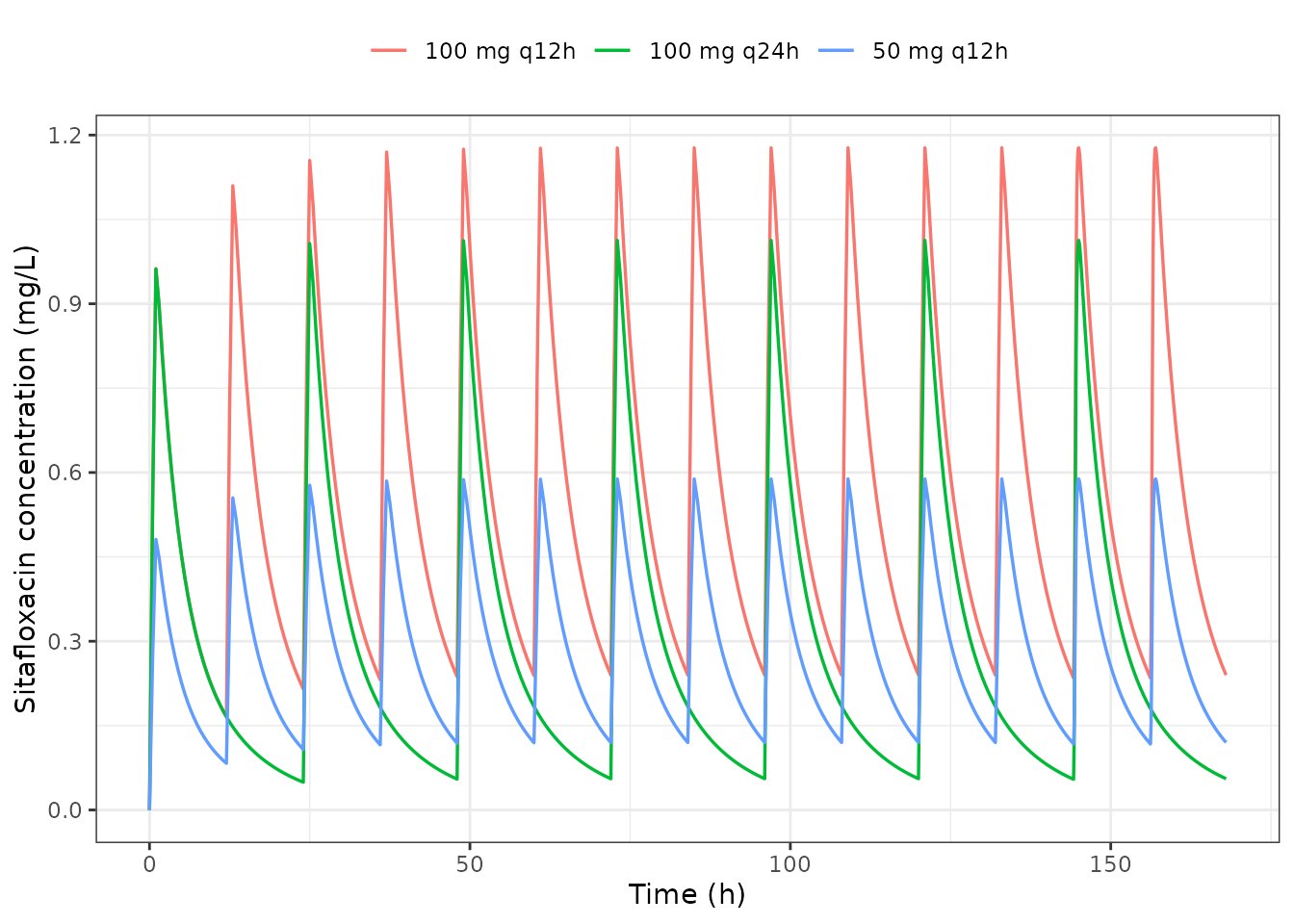

Typical-value steady-state sitafloxacin profiles for the three Wu 2025 regimens. IIV is suppressed with rxode2::zeroRe().

At the reference covariate vector (CRCL 106.88 mL/min, WT 58.55 kg, AGE 31 years, fasting) every covariate multiplier collapses to 1, so the individual parameters must equal the Table 2 typical values exactly.

ref_par <- typ |>
  dplyr::filter(regimen == "100 mg q24h") |>
  dplyr::slice(1) |>
  dplyr::select(cl, vc, vp, q, ka, d1, tlag)

published <- c(cl = 14.7, vc = 89.8, vp = 33.8, q = 5.81,
               ka = 5.19, d1 = 0.281, tlag = 0.205)

cmp_ref <- tibble::tibble(
  Parameter = names(published),
  Published = as.numeric(published),
  Simulated = round(as.numeric(ref_par[names(published)]), 4)
)
knitr::kable(cmp_ref, caption = "Typical-value parameters at the reference covariate vector vs Wu 2025 Table 2.")

Typical-value parameters at the reference covariate vector vs Wu 2025 Table 2.
Parameter	Published	Simulated
cl	14.700	14.700
vc	89.800	89.800
vp	33.800	33.800
q	5.810	5.810
ka	5.190	5.190
d1	0.281	0.281
tlag	0.205	0.205


stopifnot(all(abs(cmp_ref$Simulated - cmp_ref$Published) < 1e-6))

Absorption lag

The model applies alag(depot) <- tlag with TLAG = 0.205 h, so the concentration must be exactly zero before 0.205 h and positive afterwards.

first_dose <- typ |>
  dplyr::filter(regimen == "100 mg q24h", time <= 1)

max_conc_before_lag <- max(first_dose$Cc[first_dose$time < 0.205])
min_conc_after_lag  <- min(first_dose$Cc[first_dose$time > 0.5])

c(max_before_lag = max_conc_before_lag, min_after_lag = round(min_conc_after_lag, 4))
#> max_before_lag  min_after_lag 
#>         0.0000         0.9621
stopifnot(max_conc_before_lag == 0, min_conc_after_lag > 0)

Falsifier: the peripheral compartment is actually solved

rxSolve() defaults to useLinCmt = TRUE, which rewrites a recognisably linear system into closed form. On some two-compartment models written with micro-constants that rewrite silently drops the peripheral compartment and solves a one-compartment model instead. Total AUC is unaffected by that failure (it is still exactly dose / CL), so the AUC24h = daily dose / CL identity above cannot detect it – the only readout that moves decisively is the terminal half-life, which comes back equal to log(2) / kel.

The check below compares the simulated terminal slope against the analytic beta root of x^2 - (kel + k12 + k21) x + kel * k21 = 0 computed from the published Table 2 typical values, and prints the one-compartment value alongside so a regression is unambiguous.

hl_times <- sort(unique(c(seq(0, 4, by = 0.05), seq(4, 72, by = 0.25))))

ev_hl <- dplyr::bind_rows(
  data.frame(time = 0, amt = 100, evid = 1L, cmt = "depot", rate = -2),
  data.frame(time = hl_times, amt = NA_real_, evid = 0L, cmt = "central", rate = 0)
) |>
  dplyr::mutate(id = 1L, WT = 58.55, AGE = 31, CRCL = 106.88, FED = 0) |>
  dplyr::arrange(time, dplyr::desc(evid)) |>
  as.data.frame()

hl_sim <- rxode2::rxSolve(mod_typ, events = ev_hl, returnType = "data.frame")
#> ℹ omega/sigma items treated as zero: 'etalcl', 'etalvc', 'etald1'

# Terminal slope from the log-linear tail, well past the distribution phase.
tail_fit  <- stats::lm(log(Cc) ~ time, data = subset(hl_sim, time >= 36 & Cc > 0))
hl_simval <- log(2) / -unname(coef(tail_fit)[2])

# Analytic beta root from the published Table 2 typical values.
kel_p  <- 14.7 / 89.8
k12_p  <- 5.81 / 89.8
k21_p  <- 5.81 / 33.8
beta_p <- min(Re(polyroot(c(kel_p * k21_p, -(kel_p + k12_p + k21_p), 1))))

c(
  t_half_analytic_beta = round(log(2) / beta_p, 4),
  t_half_simulated     = round(hl_simval, 4),
  t_half_if_collapsed_to_1cmt = round(log(2) / kel_p, 4)
)
#>        t_half_analytic_beta            t_half_simulated 
#>                      7.6197                      7.6187 
#> t_half_if_collapsed_to_1cmt 
#>                      4.2343

stopifnot(
  "peripheral1 retained in the solve" = "peripheral1" %in% names(hl_sim),
  abs(hl_simval / (log(2) / beta_p) - 1) < 0.01
)

Food effect

The food effect sits entirely on the zero-order absorption duration. Because a zero-order input conserves the delivered dose, food must reshape the absorption phase (lower, later peak) while leaving the exposure over a dosing interval unchanged.

food_cohort <- tibble::tibble(
  id = 1:2, WT = 58.55, AGE = 31, CRCL = 106.88, FED = c(0, 1)
)
ev_food <- build_events(regimens[regimens$regimen == "100 mg q24h", ], food_cohort)
food <- rxode2::rxSolve(mod_typ, events = ev_food,
                        keep = c("FED"), returnType = "data.frame")
#> ℹ omega/sigma items treated as zero: 'etalcl', 'etalvc', 'etald1'
#> Warning: multi-subject simulation without without 'omega'

food_sum <- food |>
  dplyr::filter(time >= ss_start) |>
  dplyr::group_by(FED) |>
  dplyr::summarise(
    d1     = unique(round(d1, 4)),
    cmax   = max(Cc),
    tmax   = time[which.max(Cc)] - ss_start,
    auc24  = sum(diff(time) * (head(Cc, -1) + tail(Cc, -1)) / 2),
    .groups = "drop"
  ) |>
  dplyr::mutate(state = ifelse(FED == 1, "fed", "fasting"), .before = 1) |>
  dplyr::select(-FED)

knitr::kable(food_sum, digits = 4,
             caption = "Fed vs fasting at steady state (100 mg q24h, reference subject).")

Fed vs fasting at steady state (100 mg q24h, reference subject).
state	d1	cmax	tmax	auc24
fasting	0.2810	1.0128	1.0	6.8029
fed	0.8459	0.9876	1.4	6.8027


stopifnot(
  abs(food_sum$d1[food_sum$state == "fasting"] - 0.281) < 1e-3,
  abs(food_sum$d1[food_sum$state == "fed"]     - 0.846) < 1e-3,
  # Dose is conserved: AUC over the interval is unaffected by food.
  abs(diff(food_sum$auc24)) / mean(food_sum$auc24) < 0.005,
  # Cmax is reduced and Tmax delayed in the fed state.
  food_sum$cmax[food_sum$state == "fed"] < food_sum$cmax[food_sum$state == "fasting"],
  food_sum$tmax[food_sum$state == "fed"] > food_sum$tmax[food_sum$state == "fasting"]
)

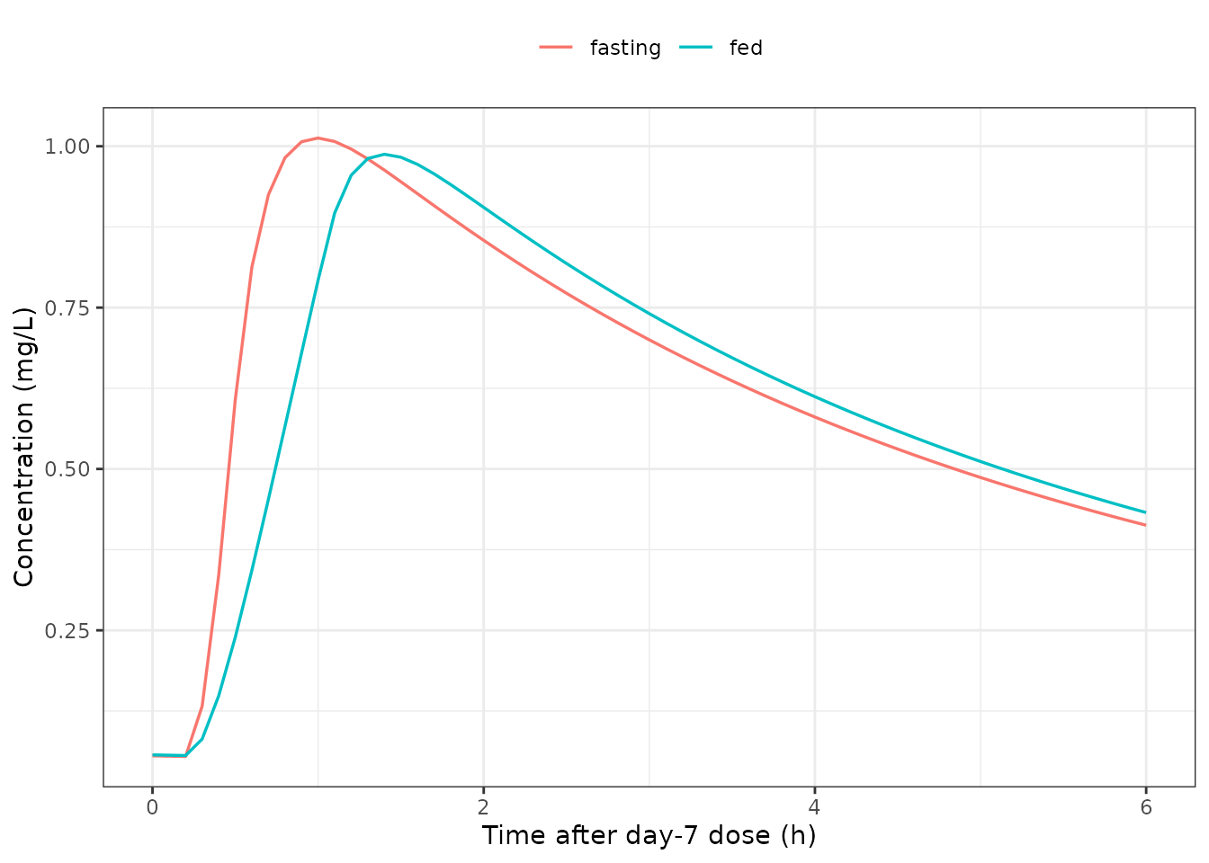
Fed vs fasting absorption phase after the day-7 dose.

NCA validation with PKNCA

Wu 2025 reports no NCA table, so there is no published Cmax/Tmax/AUC to compare against. PKNCA is still the right instrument for the quantity the paper’s PK/PD analysis is built on – the steady-state 24-hour AUC – so it is computed here over the final 24 h and then used as the falsifier below.

conc_df <- sim |>
  dplyr::filter(time >= ss_start, !is.na(Cc)) |>
  dplyr::select(id, time, Cc, regimen)

dose_df <- do.call(rbind, lapply(seq_len(nrow(regimens)), function(i) {
  r <- regimens[i, ]
  tidyr::crossing(
    tibble::tibble(id = cohort$id),
    time = seq(ss_start, t_end - r$tau, by = r$tau)
  ) |>
    dplyr::mutate(amt = r$dose, regimen = r$regimen)
})) |> as.data.frame()

conc_obj <- PKNCA::PKNCAconc(
  data = as.data.frame(conc_df),
  formula = Cc ~ time | regimen + id,
  concu = "mg/L", timeu = "h"
)
dose_obj <- PKNCA::PKNCAdose(
  data = dose_df,
  formula = amt ~ time | regimen + id,
  doseu = "mg"
)

intervals <- data.frame(
  start = ss_start, end = t_end,
  cmax = TRUE, tmax = TRUE, cmin = TRUE, auclast = TRUE, cav = TRUE
)

nca_res <- PKNCA::pk.nca(PKNCA::PKNCAdata(conc_obj, dose_obj, intervals = intervals))
nca_tbl <- as.data.frame(nca_res$result)

auc24 <- nca_tbl |>
  dplyr::filter(PPTESTCD == "auclast") |>
  dplyr::select(regimen, id, auc24_nca = PPORRES)

nca_summary <- nca_tbl |>
  dplyr::filter(PPTESTCD %in% c("cmax", "tmax", "cmin", "auclast", "cav")) |>
  dplyr::group_by(regimen, PPTESTCD) |>
  dplyr::summarise(
    median = median(PPORRES),
    p05    = quantile(PPORRES, 0.05),
    p95    = quantile(PPORRES, 0.95),
    .groups = "drop"
  ) |>
  dplyr::mutate(Parameter = nlmixr2lib::ncaParamLabel(PPTESTCD), .before = 1) |>
  dplyr::select(-PPTESTCD) |>
  dplyr::rename("Regimen" = regimen, "Median" = median,
                "5th pctile" = p05, "95th pctile" = p95)

knitr::kable(nca_summary, digits = 3,
             caption = "Simulated steady-state NCA over the final 24 h (200 subjects per regimen). Wu 2025 publishes no NCA table for comparison; these values feed the PK/PD analysis below. AUC in mg*h/L, concentrations in mg/L, times in h.")

Simulated steady-state NCA over the final 24 h (200 subjects per regimen). Wu 2025 publishes no NCA table for comparison; these values feed the PK/PD analysis below. AUC in mg*h/L, concentrations in mg/L, times in h.
Parameter	Regimen	Median	5th pctile	95th pctile
AUClast	100 mg q12h	13.760	8.156	21.143
Cavg	100 mg q12h	0.573	0.340	0.881
Cmax	100 mg q12h	1.125	0.697	1.750
Cmin	100 mg q12h	0.253	0.072	0.575
Tmax	100 mg q12h	13.000	12.800	16.610
AUClast	100 mg q24h	6.880	4.078	10.572
Cavg	100 mg q24h	0.287	0.170	0.441
Cmax	100 mg q24h	0.920	0.553	1.603
Cmin	100 mg q24h	0.058	0.012	0.198
Tmax	100 mg q24h	1.000	0.800	5.005
AUClast	50 mg q12h	6.880	4.078	10.571
Cavg	50 mg q12h	0.287	0.170	0.440
Cmax	50 mg q12h	0.562	0.349	0.875
Cmin	50 mg q12h	0.127	0.036	0.287
Tmax	50 mg q12h	13.000	12.800	16.610

Falsifier: AUC24h,ss must equal daily dose / CL, per subject

For a linear model at steady state, the exposure over 24 h is exactly the daily dose divided by the individual apparent clearance – independent of how the daily dose is split across the day, of absorption, and of food. This is a per-subject identity, which is a far stronger check than comparing cohort medians.

subj_cl <- sim |>
  dplyr::group_by(regimen, id) |>
  dplyr::summarise(cl = dplyr::first(cl), .groups = "drop")

ident <- auc24 |>
  dplyr::left_join(subj_cl, by = c("regimen", "id")) |>
  dplyr::left_join(dplyr::select(regimens, regimen, daily_dose), by = "regimen") |>
  dplyr::mutate(
    auc24_theory = daily_dose / cl,
    rel_err      = (auc24_nca - auc24_theory) / auc24_theory
  )

ident |>
  dplyr::group_by(regimen) |>
  dplyr::summarise(
    n              = dplyr::n(),
    max_abs_relerr = max(abs(rel_err)),
    .groups = "drop"
  ) |>
  dplyr::rename("Regimen" = regimen, "N subjects" = n,
                "Max |relative error|" = max_abs_relerr) |>
  knitr::kable(digits = 5,
               caption = "Per-subject agreement between the PKNCA steady-state AUC and daily dose / CL.")

Per-subject agreement between the PKNCA steady-state AUC and daily dose / CL.
Regimen	N subjects	Max \|relative error\|
100 mg q12h	200	0.00098
100 mg q24h	200	0.00098
50 mg q12h	200	0.00098


# The residual gap is trapezoidal-integration error on a 0.1 h grid, not model error.
stopifnot(nrow(ident) == n_subj * nrow(regimens), max(abs(ident$rel_err)) < 0.01)

Falsifier: equal daily doses give identical exposure

Wu 2025 reports near-identical PTAs for 50 mg q12h and 100 mg q24h (for example 99.9% and 99.9% against S. pneumoniae at the animal target). That is a consequence of both regimens delivering 100 mg/day: the 24-hour AUC must match subject by subject, and the 200 mg/day regimen must give exactly twice as much.

wide <- ident |>
  dplyr::select(regimen, id, auc24_nca) |>
  tidyr::pivot_wider(names_from = regimen, values_from = auc24_nca)

ratios <- tibble::tibble(
  Comparison = c("100 mg q24h / 50 mg q12h (equal daily dose)",
                 "100 mg q12h / 50 mg q12h (double daily dose)"),
  `Median ratio` = c(
    median(wide$`100 mg q24h` / wide$`50 mg q12h`),
    median(wide$`100 mg q12h` / wide$`50 mg q12h`)
  ),
  `Max deviation` = c(
    max(abs(wide$`100 mg q24h` / wide$`50 mg q12h` - 1)),
    max(abs(wide$`100 mg q12h` / wide$`50 mg q12h` - 2))
  )
)
knitr::kable(ratios, digits = 5,
             caption = "Per-subject steady-state AUC ratios between regimens.")

Per-subject steady-state AUC ratios between regimens.
Comparison	Median ratio	Max deviation
100 mg q24h / 50 mg q12h (equal daily dose)	1	0.00016
100 mg q12h / 50 mg q12h (double daily dose)	2	0.00000


stopifnot(
  max(abs(wide$`100 mg q24h` / wide$`50 mg q12h` - 1)) < 0.01,
  max(abs(wide$`100 mg q12h` / wide$`50 mg q12h` - 2)) < 0.02
)

Falsifier: the covariate relationships are recovered

Regressing each log parameter on its log covariates should return the published exponents. The estimates are not noise-free: the IIV terms (omega = 0.23 on CL, 0.25 on V2) act as residual error in these regressions, so each recovered exponent carries a genuine sampling standard error. With 200 subjects that error is about 0.04 for the CRCL and AGE exponents and about 0.11 for the WT exponent – body weight has the narrowest spread of the three covariates (sd(log(WT)) around 0.18 versus 0.48 for age), so its exponent is the least precisely identified.

A fixed absolute tolerance would therefore be a seed lottery rather than a test. The check below is calibrated to the regression’s own uncertainty instead: each published exponent must fall inside the fitted 95% confidence interval, and must be within 3 standard errors of the estimate. A second assertion bounds the standard errors themselves, so the test retains the power to fail – without it, a degenerate cohort with huge standard errors would pass the coverage check vacuously.

par_by_subj <- sim |>
  dplyr::filter(regimen == "100 mg q24h") |>
  dplyr::group_by(id) |>
  dplyr::summarise(
    cl = dplyr::first(cl), vc = dplyr::first(vc),
    CRCL = dplyr::first(CRCL), WT = dplyr::first(WT), AGE = dplyr::first(AGE),
    .groups = "drop"
  )

# CL has one covariate, so regressing log CL on log CRCL recovers the exponent
# up to the eta noise. Vc has two, so both exponents come from one regression.
fit_cl <- stats::lm(log(cl) ~ log(CRCL), data = par_by_subj)
fit_vc <- stats::lm(log(vc) ~ log(WT) + log(AGE), data = par_by_subj)

# (fit, coefficient index) for each published relationship.
fits <- list(list(fit_cl, 2L), list(fit_vc, 2L), list(fit_vc, 3L))

recovery <- tibble::tibble(
  Relationship = c("CRCL on CL/F", "WT on V2/F", "AGE on V2/F"),
  Published    = c(0.460, 0.966, 0.286),
  Recovered    = vapply(fits, function(f) unname(coef(f[[1]])[f[[2]]]), numeric(1)),
  StdError     = vapply(fits, function(f) summary(f[[1]])$coefficients[f[[2]], 2], numeric(1)),
  CIlow        = vapply(fits, function(f) confint(f[[1]])[f[[2]], 1], numeric(1)),
  CIhigh       = vapply(fits, function(f) confint(f[[1]])[f[[2]], 2], numeric(1))
) |>
  dplyr::mutate(
    ZfromPublished = abs(Recovered - Published) / StdError,
    PublishedInCI  = Published >= CIlow & Published <= CIhigh
  )

recovery |>
  dplyr::rename(
    "Published" = Published, "Recovered" = Recovered, "SE" = StdError,
    "95% CI lower" = CIlow, "95% CI upper" = CIhigh,
    "|est - pub| / SE" = ZfromPublished, "Published in CI" = PublishedInCI
  ) |>
  knitr::kable(digits = 4,
               caption = "Covariate exponents recovered from the simulated cohort vs Wu 2025 Table 2, with the sampling uncertainty of each regression coefficient.")

Covariate exponents recovered from the simulated cohort vs Wu 2025 Table 2, with the sampling uncertainty of each regression coefficient.
Relationship	Published	Recovered	SE	95% CI lower	95% CI upper	\|est - pub\| / SE	Published in CI
CRCL on CL/F	0.460	0.4906	0.0409	0.4098	0.5713	0.7463	TRUE
WT on V2/F	0.966	1.0884	0.1102	0.8710	1.3057	1.1103	TRUE
AGE on V2/F	0.286	0.2468	0.0405	0.1670	0.3266	0.9691	TRUE


stopifnot(
  # Every published exponent is covered by its own 95% confidence interval, and
  # sits within 3 SE of the point estimate.
  all(recovery$PublishedInCI),
  all(recovery$ZfromPublished < 3),
  # Power guard: the standard errors must stay small enough that a materially
  # wrong exponent would be rejected above rather than absorbed into a wide CI.
  all(recovery$StdError < 0.15)
)

PK/PD cut-offs (Wu 2025 Tables 3 and 4)

This is the paper’s headline result and the strongest available answer key: 12 PK/PD cut-off cells and 12 PTA values across three regimens and four pathogen-specific targets.

The PK/PD index is the unbound fAUC24h/MIC. Wu 2025 never reports a sitafloxacin unbound fraction. The value used here, fu = 0.388, is not from Wu 2025: it is carried from the separately packaged Rodjun_2023_sitafloxacin model, where Rodjun 2023 sources it to Tanigawara 2013. It is applied only in this section, never inside the model file.

fu <- 0.388   # NOT from Wu 2025. Rodjun 2023 Methods, sourced there to Tanigawara 2013.
rodjun <- readModelDb("Rodjun_2023_sitafloxacin")()
grep("0.388", rodjun$description, value = TRUE) |> substr(1, 200)
#> [1] "Population PK model for oral sitafloxacin as encoded by Rodjun 2023 for Monte Carlo probability-of-target-attainment simulation against carbapenem-, multidrug- and colistin-resistant Acinetobacter bau"

Because AUC24h,ss = daily dose / CL holds exactly per subject (verified above), the probability of target attainment can be evaluated on a large sample of individual clearances without re-solving the ODE system. That buys the precision Wu 2025’s Monte Carlo had – their PTAs are quoted to 0.1%, which 200 simulated subjects cannot resolve – at negligible cost.

n_mc <- 10000L

set.seed(4620)
mc <- tibble::tibble(
  CRCL = draw_crcl(n_mc),
  eta  = stats::rnorm(n_mc, 0, sqrt(0.0515))
) |>
  dplyr::mutate(cl = 14.7 * (CRCL / 106.88)^0.460 * exp(eta))

# Sanity: the closed form must agree with the ODE cohort's clearance distribution.
c(ode_median_cl = median(par_by_subj$cl), mc_median_cl = median(mc$cl))
#> ode_median_cl  mc_median_cl 
#>      14.53500      14.83822
stopifnot(abs(median(mc$cl) / median(par_by_subj$cl) - 1) < 0.10)

pta <- function(daily_dose, mic, target) {
  mean(fu * daily_dose / mc$cl / mic >= target)
}

mic_grid <- c(0.008, 0.015, 0.03, 0.06, 0.125, 0.25, 0.5, 1, 2, 4)

targets <- tibble::tribble(
  ~scenario,                                        ~target,
  "S. pneumoniae, animal model (fAUC24h/MIC 11.56)",  11.56,
  "S. pneumoniae, clinical (fAUC24h/MIC >= 30)",      30.00,
  "S. aureus, animal model (fAUC24h/MIC 18.32)",      18.32,
  "Gram-negatives, animal model (fAUC24h/MIC 15.06)", 15.06
)

pta_grid <- tidyr::crossing(targets, regimens, mic = mic_grid) |>
  dplyr::mutate(pta = mapply(pta, daily_dose, mic, target) * 100)

ggplot(pta_grid, aes(mic, pta, colour = regimen)) +
  geom_line(linewidth = 0.6) +
  geom_point(size = 1) +
  geom_hline(yintercept = 95, linetype = "dashed") +
  scale_x_log10(breaks = mic_grid, labels = mic_grid) +
  facet_wrap(~scenario, ncol = 2) +
  labs(x = "MIC (mg/L)", y = "PTA (%)", colour = NULL) +
  theme_bw() +
  theme(legend.position = "top", axis.text.x = element_text(angle = 45, hjust = 1))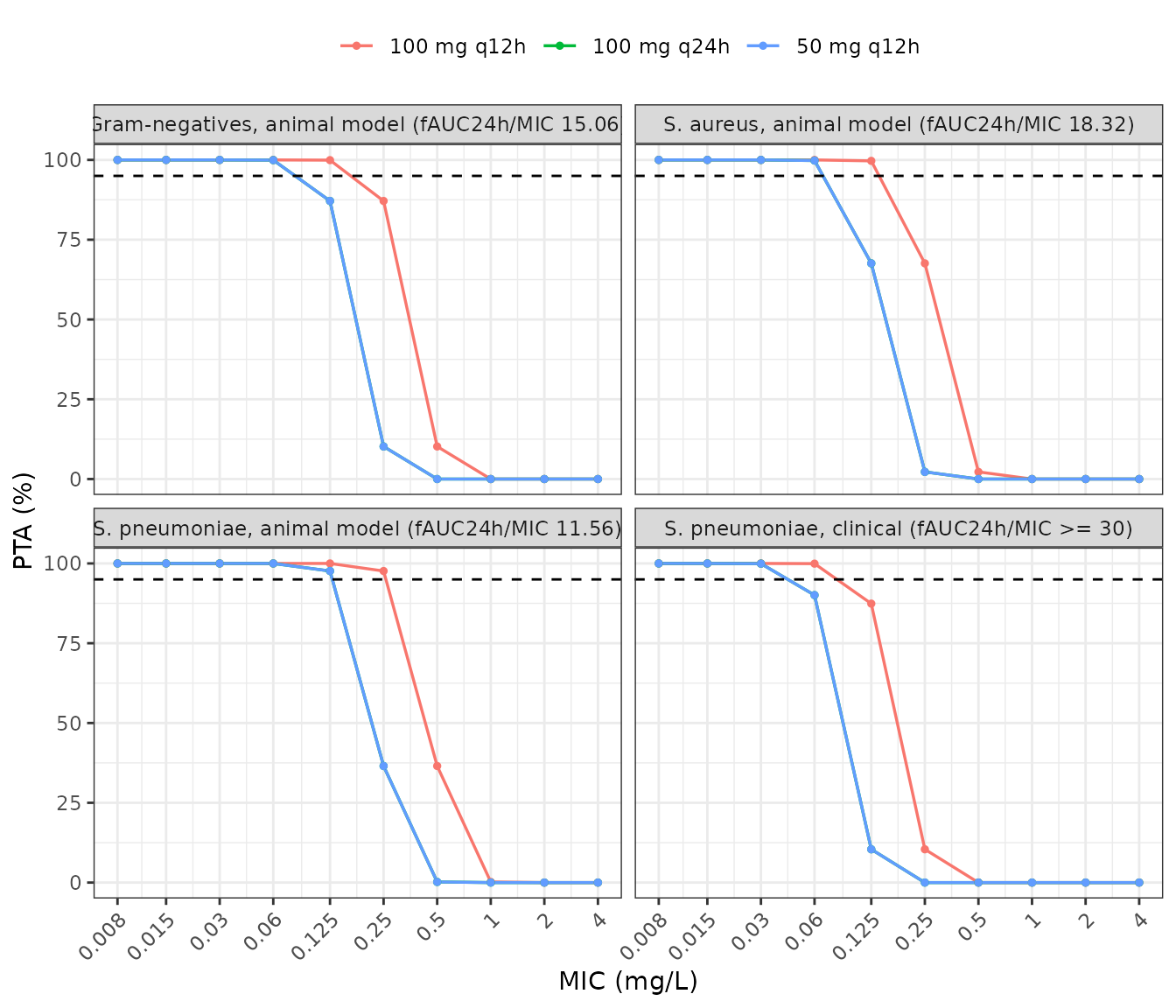

Replicates Wu 2025 Figure 3: probability of target attainment versus MIC for the three dosing regimens, by PK/PD target. Dashed line marks the 95% PTA criterion.

Comparison against the published cut-offs

Wu 2025 Section 4.2 defines the cut-off as “the highest value of the corresponding MIC range” at which the PTA exceeds 95%.

simulated_cutoffs <- pta_grid |>
  dplyr::filter(pta >= 95) |>
  dplyr::group_by(scenario, regimen) |>
  dplyr::summarise(
    cutoff_sim = max(mic),
    pta_at_cutoff_sim = pta[which.max(mic)],
    .groups = "drop"
  )

# Wu 2025 Table 3, transcribed. Every cell of the published table is represented.
published_cutoffs <- tibble::tribble(
  ~scenario,                                          ~regimen,       ~cutoff_pub, ~pta_pub,
  "S. pneumoniae, animal model (fAUC24h/MIC 11.56)",  "50 mg q12h",    0.06,        99.9,
  "S. pneumoniae, animal model (fAUC24h/MIC 11.56)",  "100 mg q24h",   0.06,        99.9,
  "S. pneumoniae, animal model (fAUC24h/MIC 11.56)",  "100 mg q12h",   0.125,       99.7,
  "S. pneumoniae, clinical (fAUC24h/MIC >= 30)",      "50 mg q12h",    0.03,        99.3,
  "S. pneumoniae, clinical (fAUC24h/MIC >= 30)",      "100 mg q24h",   0.03,        99.1,
  "S. pneumoniae, clinical (fAUC24h/MIC >= 30)",      "100 mg q12h",   0.06,        99.1,
  "S. aureus, animal model (fAUC24h/MIC 18.32)",      "50 mg q12h",    0.06,        97.7,
  "S. aureus, animal model (fAUC24h/MIC 18.32)",      "100 mg q24h",   0.06,        97.9,
  "S. aureus, animal model (fAUC24h/MIC 18.32)",      "100 mg q12h",   0.125,       97.0,
  "Gram-negatives, animal model (fAUC24h/MIC 15.06)", "50 mg q12h",    0.06,        99.3,
  "Gram-negatives, animal model (fAUC24h/MIC 15.06)", "100 mg q24h",   0.06,        99.1,
  "Gram-negatives, animal model (fAUC24h/MIC 15.06)", "100 mg q12h",   0.125,       98.8
)

cutoff_cmp <- published_cutoffs |>
  dplyr::left_join(simulated_cutoffs, by = c("scenario", "regimen")) |>
  dplyr::mutate(
    dilutions_off = round(log2(cutoff_sim / cutoff_pub)),
    agree = ifelse(dilutions_off == 0, "yes", paste0(dilutions_off, " dilution"))
  )

# Guard against a silently empty join: every published cell must have matched.
stopifnot(nrow(cutoff_cmp) == 12L, !anyNA(cutoff_cmp$cutoff_sim))

cutoff_cmp |>
  dplyr::select(scenario, regimen, cutoff_pub, cutoff_sim,
                pta_pub, pta_at_cutoff_sim, agree) |>
  dplyr::rename(
    "Scenario" = scenario, "Regimen" = regimen,
    "Cut-off, Wu 2025 (mg/L)" = cutoff_pub,
    "Cut-off, simulated (mg/L)" = cutoff_sim,
    "PTA at cut-off, Wu 2025 (%)" = pta_pub,
    "PTA at cut-off, simulated (%)" = pta_at_cutoff_sim,
    "Agreement" = agree
  ) |>
  knitr::kable(digits = 1,
               caption = "Simulated vs published PK/PD cut-offs and PTAs (Wu 2025 Table 3).")

Simulated vs published PK/PD cut-offs and PTAs (Wu 2025 Table 3).
Scenario	Regimen	Cut-off, Wu 2025 (mg/L)	Cut-off, simulated (mg/L)	PTA at cut-off, Wu 2025 (%)	PTA at cut-off, simulated (%)	Agreement
S. pneumoniae, animal model (fAUC24h/MIC 11.56)	50 mg q12h	0.1	0.1	99.9	97.6	1 dilution
S. pneumoniae, animal model (fAUC24h/MIC 11.56)	100 mg q24h	0.1	0.1	99.9	97.6	1 dilution
S. pneumoniae, animal model (fAUC24h/MIC 11.56)	100 mg q12h	0.1	0.2	99.7	97.6	1 dilution
S. pneumoniae, clinical (fAUC24h/MIC >= 30)	50 mg q12h	0.0	0.0	99.3	99.9	yes
S. pneumoniae, clinical (fAUC24h/MIC >= 30)	100 mg q24h	0.0	0.0	99.1	99.9	yes
S. pneumoniae, clinical (fAUC24h/MIC >= 30)	100 mg q12h	0.1	0.1	99.1	99.9	yes
S. aureus, animal model (fAUC24h/MIC 18.32)	50 mg q12h	0.1	0.1	97.7	99.8	yes
S. aureus, animal model (fAUC24h/MIC 18.32)	100 mg q24h	0.1	0.1	97.9	99.8	yes
S. aureus, animal model (fAUC24h/MIC 18.32)	100 mg q12h	0.1	0.1	97.0	99.7	yes
Gram-negatives, animal model (fAUC24h/MIC 15.06)	50 mg q12h	0.1	0.1	99.3	99.9	yes
Gram-negatives, animal model (fAUC24h/MIC 15.06)	100 mg q24h	0.1	0.1	99.1	99.9	yes
Gram-negatives, animal model (fAUC24h/MIC 15.06)	100 mg q12h	0.1	0.1	98.8	99.9	yes


n_exact <- sum(cutoff_cmp$dilutions_off == 0)
cat(sprintf("%d of 12 cells reproduce the published cut-off exactly; %d of 12 within one doubling dilution.\n",
            n_exact, sum(abs(cutoff_cmp$dilutions_off) <= 1)))
#> 9 of 12 cells reproduce the published cut-off exactly; 12 of 12 within one doubling dilution.

The published cut-offs also have an internal structure worth testing directly. MIC values are reported on a doubling-dilution series whose printed labels are conventionally rounded (0.008, 0.015, 0.03, 0.06, 0.125, 0.25, ...), so “one dilution higher” is not a numeric ratio of exactly 2 – the step from 0.06 to 0.125 is a factor of 2.083. The relationships between regimens are therefore tested as positions in the dilution series rather than as ratios.

# Position of a printed MIC in the doubling-dilution series.
dil_index <- function(mic) match(mic, mic_grid)

step_check <- cutoff_cmp |>
  dplyr::select(scenario, regimen, cutoff_pub) |>
  tidyr::pivot_wider(names_from = regimen, values_from = cutoff_pub) |>
  dplyr::mutate(
    step_double_daily_dose = dil_index(`100 mg q12h`) - dil_index(`50 mg q12h`),
    step_equal_daily_dose  = dil_index(`100 mg q24h`) - dil_index(`50 mg q12h`)
  )

step_check |>
  dplyr::select(scenario, step_double_daily_dose, step_equal_daily_dose) |>
  dplyr::rename(
    "Scenario" = scenario,
    "Dilutions: 100 q12h vs 50 q12h (2x daily dose)" = step_double_daily_dose,
    "Dilutions: 100 q24h vs 50 q12h (same daily dose)" = step_equal_daily_dose
  ) |>
  knitr::kable(caption = "Internal structure of the Wu 2025 Table 3 cut-offs, in doubling dilutions.")

Internal structure of the Wu 2025 Table 3 cut-offs, in doubling dilutions.
Scenario	Dilutions: 100 q12h vs 50 q12h (2x daily dose)	Dilutions: 100 q24h vs 50 q12h (same daily dose)
S. pneumoniae, animal model (fAUC24h/MIC 11.56)	1	0
S. pneumoniae, clinical (fAUC24h/MIC >= 30)	1	0
S. aureus, animal model (fAUC24h/MIC 18.32)	1	0
Gram-negatives, animal model (fAUC24h/MIC 15.06)	1	0


stopifnot(
  # A doubling-dilution series is the resolution of the published answer key, so
  # agreement to within one dilution across every cell is the meaningful bar.
  all(abs(cutoff_cmp$dilutions_off) <= 1),
  nrow(step_check) == 4L,
  # Doubling the daily dose moves the published cut-off exactly one dilution up.
  all(step_check$step_double_daily_dose == 1L),
  # Equal daily doses split differently give exactly the same cut-off, which is
  # the same identity the per-subject AUC check established above.
  all(step_check$step_equal_daily_dose == 0L)
)

Assumptions and deviations

Errata and open items

eta4 (inter-occasion variability) is not encoded. Wu 2025 Table 2 reports a fourth random effect with omega^2 = 0.0279 (RSE 8.7%, shrinkage 29.1%, bootstrap 95% CI 0.0184-0.0394). The abbreviation footnote describes it only as “eta4, interindividual variability of IOV” and never names the structural parameter it acts on; the Section 2.2 display equations account for eta1, eta2 and eta3 only. No supplement or control stream is available (the EuropePMC supplementaryFiles endpoint returns HTTP 500 for PMC11868765 and the Frontiers file endpoints return 404), and the supplement’s documented contents – a study-design table and mean concentration-time figures – would not place an eta. Assigning the term to CL, D1 or F would be inventing model structure, so it is omitted and its reported value preserved in the model file comments. Simulated between-subject spread in AUC is therefore marginally narrower than the paper’s, which if anything makes the PTAs above slightly optimistic at the extremes.
The unbound fraction is not from Wu 2025. fu = 0.388 used in the PK/PD section is carried from Rodjun_2023_sitafloxacin (Rodjun 2023 Methods, sourced there to Tanigawara 2013). Wu 2025 computes fAUC24h/MIC throughout but never states the unbound fraction it used. The model file deliberately does not carry an fu term.
CFR is not reproduced. Wu 2025 Table 3 also reports cumulative fraction of response, which requires the EUCAST MIC frequency distributions for each pathogen. Those distributions are external to the paper and are not on disk, so only the PTA and cut-off columns are validated here.
No NCA answer key. Wu 2025 publishes no Cmax/Tmax/AUC table, so the PKNCA results above are reported rather than compared, and the validation weight rests on the per-subject AUC24h = daily dose / CL identity and the PK/PD cut-off table.
eta3 on D1 is extreme as published (omega^2 = 3.46, i.e. omega = 1.86 on the log scale). It is encoded exactly as reported. Because a zero-order input conserves the delivered dose, even large eta3 draws leave AUC – and therefore every PK/PD conclusion – untouched, perturbing only Cmax and Tmax.

Assumptions made because the paper does not say

Covariate distributions. Wu 2025 Table 1 reports only marginal mean +/- SD. Age, weight and creatinine clearance are drawn here as independent log-normals moment-matched to those marginals. Real cohorts correlate age, weight and renal function; ignoring that correlation is the largest single approximation in the PTA reproduction.
Renal-function floor. Creatinine clearance is truncated at 50 mL/min per Wu 2025 Section 4.2. The paper does not state the shape of the CRCL distribution it simulated from.
Reference values. The normalizing constants 106.88 mL/min, 58.55 kg and 31 years are printed inside the Section 2.2 equations but never labelled. They are close to, yet distinct from, the Table 1 means, and are most likely medians. They are used exactly as printed.
Fed state in the PK/PD simulations. Wu 2025 does not state whether the simulated subjects were fed or fasting. The cohort is simulated fasting (FED = 0). This has no effect on any conclusion: the food effect acts only on the zero-order absorption duration, which the food-effect section above shows leaves the 24-hour AUC unchanged.
Cut-off criterion. Wu 2025 says the PTA must be “greater than 95%”; a >= 95% rule is used here. No cell in the table sits close enough to 95% for the distinction to matter. ```